- Packages in R for principal component analysis
- prcomp() and princomp() functions
- Install factoextra for visualization
- Prepare the data
- Use the R function prcomp() for PCA
- Variances of the principal components
- Graph of variables : The correlation circle
- Graph of individuals
- Prediction using Principal Component Analysis
- Infos
The basics of Principal Component Analysis (PCA) have been already described in my previous article : PCA basics.
This R tutorial describes how to perform a Principal Component Analysis (PCA) using the built-in R functions prcomp() and princomp().
You will learn how to :
- determine the number of components to retain for summarizing the information in your data
- calculate the coordinates, the cos2 and the contribution of variables
- calculate the coordinates, the cos2 and the contribution of individuals
- interpret the correlation circle of PCA
- make a prediction with PCA
Packages in R for principal component analysis
There are two general methods to perform PCA in R :
- Spectral decomposition which examines the covariances / correlations between variables
- Singular value decomposition which examines the covariances / correlations between individuals
The singular value decomposition method is the preferred analysis for numerical accuracy.
There are several functions from different packages for performing PCA :
- The functions prcomp() and princomp() from the built-in R stats package
- PCA() from FactoMineR package. Read more here : PCA with FactoMineR
- dudi.pca() from ade4 package. Read more here : PCA with ade4
The functions prcomp() and princomp() are described in the next section.
prcomp() and princomp() functions
The function princomp() uses the spectral decomposition approach.
The functions prcomp() and PCA()[FactoMineR] use the singular value decomposition (SVD).
According to R help, SVD has slightly better numerical accuracy. Therefore, prcomp() is the preferred function.
The simplified format of these 2 functions are :
prcomp(x, scale = FALSE)

princomp(x, cor = FALSE, scores = TRUE)- Arguments for prcomp() :
- x : a numeric matrix or data frame
- scale : a logical value indicating whether the variables should be scaled to have unit variance before the analysis takes place
- Arguments for princomp() :
- x : a numeric matrix or data frame
- cor : a logical value. If TRUE, the data will be centered and scaled before the analysis
- scores : a logical value. If TRUE, the coordinates on each principal component are calculated
The elements of the outputs returned by the functions prcomp() and princomp() includes :
| prcomp() name | princomp() name | Description |
|---|---|---|
| sdev | sdev | the standard deviations of the principal components |
| rotation | loadings | the matrix of variable loadings (columns are eigenvectors) |
| center | center | the variable means (means that were substracted) |
| scale | scale | the variable standard deviations (the scalings applied to each variable ) |
| x | scores | The coordinates of the individuals (observations) on the principal components. |
In the following sections, well focus only on the function prcomp()
Install factoextra for visualization
The package factoextra is used for the visualization of the principal component analysis results.
factoextra can be installed and loaded as follow :
# install.packages("devtools")
devtools::install_github("kassambara/factoextra")

# load
library("factoextra")
Prepare the data
Well use the data sets decathlon2 from the package factoextra :
library("factoextra")
data(decathlon2)
This data is a subset of decathlon data in FactoMineR package
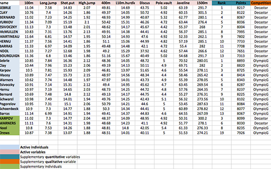
As illustrated below, the data used here describes athletes performance during two sporting events (Desctar and OlympicG). It contains 27 individuals (athletes) described by 13 variables :
Only some of these individuals and variables will be used to perform the principal component analysis (PCA).
The coordinates of the remaining individuals and variables on the factor map will be predicted after the PCA.In PCA terminology, our data contains :
- Active individuals (in blue, rows 1:23) : Individuals that are used during the principal component analysis.
- Supplementary individuals (in green, rows 24:27) : The coordinates of these individuals will be predicted using the PCA information and parameters obtained with active individuals/variables
- Active variables (in pink, columns 1:10) : Variables that are used for the principal component analysis.
- Supplementary variables : As supplementary individuals, the coordinates of these variables will be predicted also.
- Supplementary continuous variables : Columns 11 and 12 corresponding respectively to the rank and the points of athletes.
- Supplementary qualitative variables : Column 13 corresponding to the two athletic meetings (2004 Olympic Game or 2004 Decastar). This factor variables will be used to color individuals by groups.
Extract only active individuals and variables for principal component analysis:
decathlon2.active <- decathlon2[1:23, 1:10]
head(decathlon2.active[, 1:6])
X100m Long.jump Shot.put High.jump X400m X110m.hurdle
SEBRLE 11.04 7.58 14.83 2.07 49.81 14.69
CLAY 10.76 7.40 14.26 1.86 49.37 14.05
BERNARD 11.02 7.23 14.25 1.92 48.93 14.99
YURKOV 11.34 7.09 15.19 2.10 50.42 15.31
ZSIVOCZKY 11.13 7.30 13.48 2.01 48.62 14.17
McMULLEN 10.83 7.31 13.76 2.13 49.91 14.38Use the R function prcomp() for PCA
res.pca <- prcomp(decathlon2.active, scale = TRUE)The values returned, by the function prcomp(), are :
names(res.pca)[1] "sdev" "rotation" "center" "scale" "x" - sdev : the standard deviations of the principal components (the square roots of the eigenvalues)
head(res.pca$sdev)[1] 2.0308159 1.3559244 1.1131668 0.9052294 0.8375875 0.6502944- rotation : the matrix of variable loadings (columns are eigenvectors)
head(unclass(res.pca$rotation)[, 1:4]) PC1 PC2 PC3 PC4
X100m -0.4188591 0.13230683 -0.2708996 0.03708806
Long.jump 0.3910648 -0.20713320 0.1711752 -0.12746997
Shot.put 0.3613881 -0.06298590 -0.4649778 0.14191803
High.jump 0.3004132 0.34309742 -0.2965280 0.15968342
X400m -0.3454786 -0.21400770 -0.2547084 0.47592968
X110m.hurdle -0.3762651 0.01824645 -0.4032525 -0.01866477- center, scale : the centering and scaling used, or FALSE
Variances of the principal components
The variance retained by each principal component can be obtained as follow :
# Eigenvalues
eig <- (res.pca$sdev)^2

# Variances in percentage
variance <- eig*100/sum(eig)

# Cumulative variances
cumvar <- cumsum(variance)

eig.decathlon2.active <- data.frame(eig = eig, variance = variance,
                     cumvariance = cumvar)
head(eig.decathlon2.active)
eig variance cumvariance
1 4.1242133 41.242133 41.24213
2 1.8385309 18.385309 59.62744
3 1.2391403 12.391403 72.01885
4 0.8194402 8.194402 80.21325
5 0.7015528 7.015528 87.22878
6 0.4228828 4.228828 91.45760Note that, you can use the function summary() to extract the eigenvalues and variances from an object of class prcomp.
summary(res.pca)You can also use the package factoextra. Its simple :
library("factoextra")
eig.val <- get_eigenvalue(res.pca)
head(eig.val)
eigenvalue variance.percent cumulative.variance.percent
Dim.1 4.1242133 41.242133 41.24213
Dim.2 1.8385309 18.385309 59.62744
Dim.3 1.2391403 12.391403 72.01885
Dim.4 0.8194402 8.194402 80.21325
Dim.5 0.7015528 7.015528 87.22878
Dim.6 0.4228828 4.228828 91.45760What mean eigenvalues ?
Recall that eigenvalues measures the variability retained by each PC. Its large for the first PC and small for the subsequent PCs.
The importance of princpal components (PCs) can be visualized with a scree plot.
Scree plot using base graphics :
barplot(eig.decathlon2.active[, 2], names.arg=1:nrow(eig.decathlon2.active),
       main = "Variances",
       xlab = "Principal Components",
       ylab = "Percentage of variances",
       col ="steelblue")
# Add connected line segments to the plot
lines(x = 1:nrow(eig.decathlon2.active),
      eig.decathlon2.active[, 2],
      type="b", pch=19, col = "red")
~60% of the information (variances) contained in the data are retained by the first two principal components.
Scree plot using factoextra :
fviz_screeplot(res.pca, ncp=10)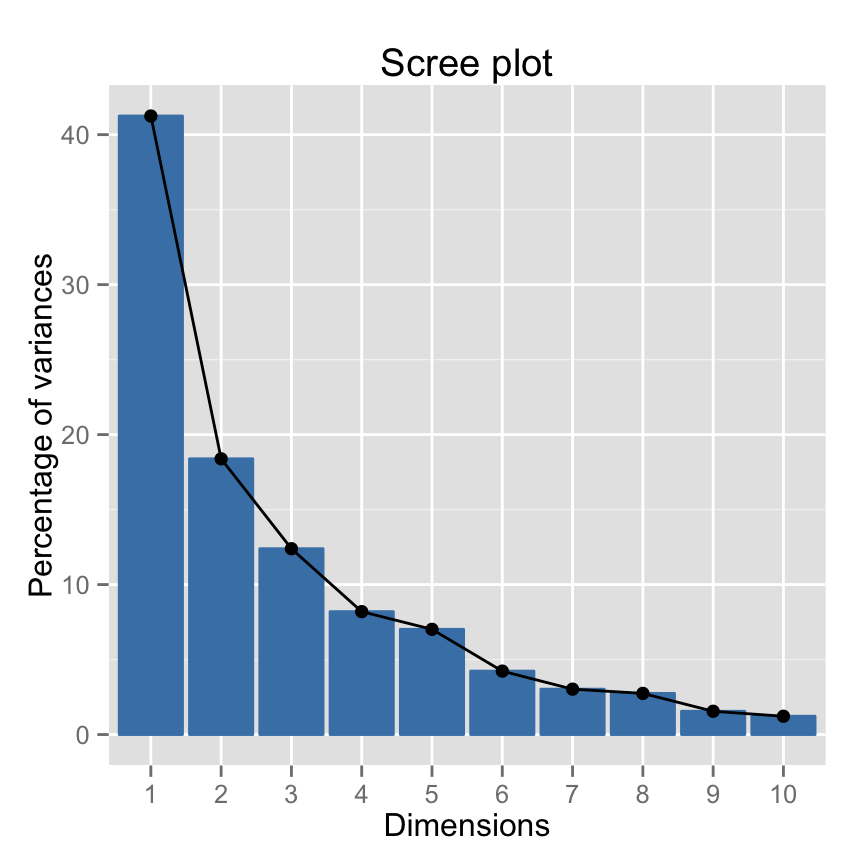
Its also possible to visualize the eigenvalues instead of the variances :
fviz_screeplot(res.pca, ncp=10, choice="eigenvalue")
Read more about fviz_screeplot.
How to determine the number of components to retain?
- An eigenvalue> 1 indicates that PCs account for more variance than accounted by one of the original variables in standardized data. This is commonly used as a cutoff point for which PCs are retained.
- You can also limit the number of component to that number that accounts for a certain fraction of the total variance. For example, if you are satisfied with 80% of the total variance explained then use the number of components to achieve that.
Note that, a good dimension reduction is achieved when the the first few PCs account for a large proportion of the variability (80-90%).
Graph of variables : The correlation circle
A simple method to extract the results, for variables, from a PCA output is to use the function get_pca_var() [factoextra]. This function provides a list of matrices containing all the results for the active variables (coordinates, correlation between variables and axes, squared cosine and contributions)
var <- get_pca_var(res.pca)
var
Principal Component Analysis Results for variables
===================================================
Name Description
1 "$coord" "Coordinates for the variables"
2 "$cor" "Correlations between variables and dimensions"
3 "$cos2" "Cos2 for the variables"
4 "$contrib" "contributions of the variables" # Coordinates of variables
var$coord[, 1:4] Dim.1 Dim.2 Dim.3 Dim.4
X100m -0.850625692 0.17939806 -0.30155643 0.03357320
Long.jump 0.794180641 -0.28085695 0.19054653 -0.11538956
Shot.put 0.733912733 -0.08540412 -0.51759781 0.12846837
High.jump 0.610083985 0.46521415 -0.33008517 0.14455012
X400m -0.701603377 -0.29017826 -0.28353292 0.43082552
X110m.hurdle -0.764125197 0.02474081 -0.44888733 -0.01689589
Discus 0.743209016 -0.04966086 -0.17652518 0.39500915
Pole.vault -0.217268042 -0.80745110 -0.09405773 -0.33898477
Javeline 0.428226639 -0.38610928 -0.60412432 -0.33173454
X1500m 0.004278487 -0.78448019 0.21947068 0.44800961In this section Ill show you, step by step, how to calculate the coordinates, the cos2 and the contribution of variables.
Coordinates of variables on the principal components
The correlation between variables and principal components is used as coordinates. It can be calculated as follow :
Variable correlations with PCs = loadings * the component standard deviations.
# Helper function :
# Correlation between variables and principal components
var_cor_func <- function(var.loadings, comp.sdev){
  var.loadings*comp.sdev
  }

# Variable correlation/coordinates
loadings <- res.pca$rotation
sdev <- res.pca$sdev

var.coord <- var.cor <- t(apply(loadings, 1, var_cor_func, sdev))
head(var.coord[, 1:4])
PC1 PC2 PC3 PC4
X100m -0.8506257 0.17939806 -0.3015564 0.03357320
Long.jump 0.7941806 -0.28085695 0.1905465 -0.11538956
Shot.put 0.7339127 -0.08540412 -0.5175978 0.12846837
High.jump 0.6100840 0.46521415 -0.3300852 0.14455012
X400m -0.7016034 -0.29017826 -0.2835329 0.43082552
X110m.hurdle -0.7641252 0.02474081 -0.4488873 -0.01689589Graph of variables using R base graph
# Plot the correlation circle
a <- seq(0, 2*pi, length = 100)
plot( cos(a), sin(a), type = 'l', col="gray",
      xlab = "PC1",  ylab = "PC2")

abline(h = 0, v = 0, lty = 2)

# Add active variables
arrows(0, 0, var.coord[, 1], var.coord[, 2],
      length = 0.1, angle = 15, code = 2)

# Add labels
text(var.coord, labels=rownames(var.coord), cex = 1, adj=1)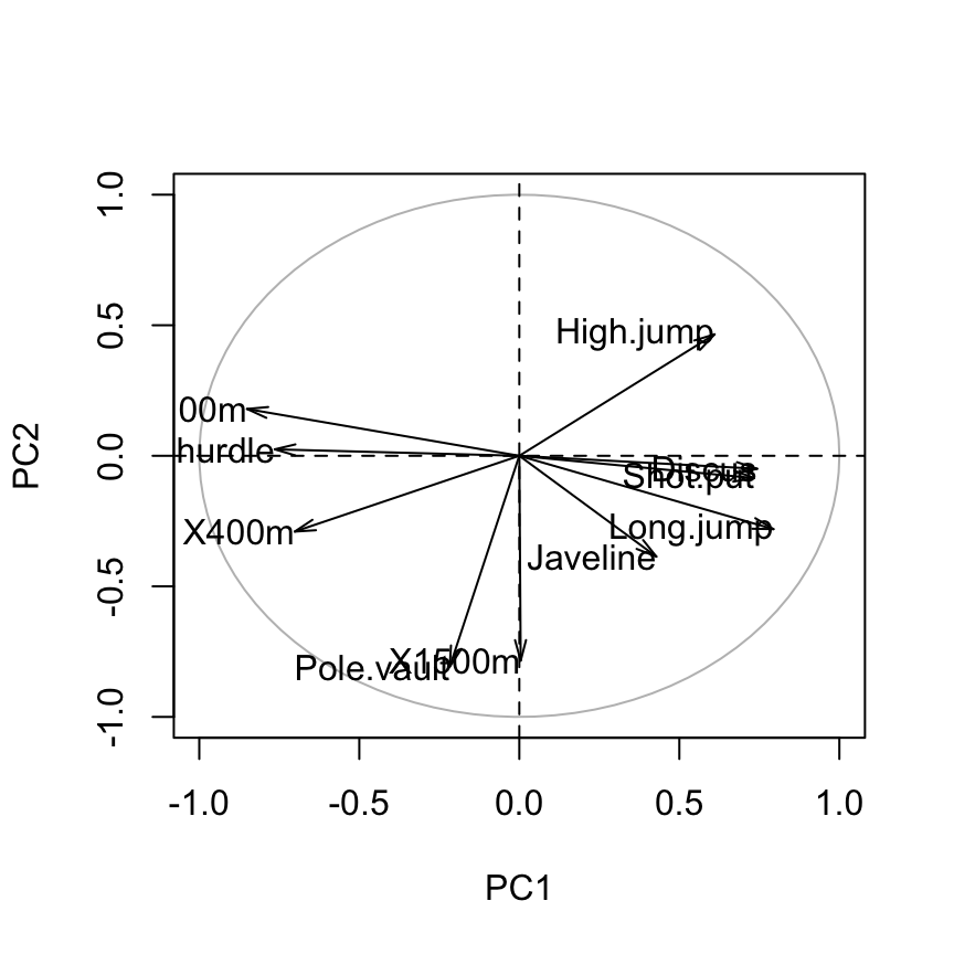
Graph of variables using factoextra
fviz_pca_var(res.pca)
Read more about the function fviz_pca_var() : Graph of variables - Principal Component Analysis
How to interpret the correlation plot?
The graph of variables shows the relationships between all variables :
- Positively correlated variables are grouped together.
- Negatively correlated variables are positioned on opposite sides of the plot origin (opposed quadrants).
- The distance between variables and the origine measures the quality of the variables on the factor map. Variables that are away from the origin are well represented on the factor map.
Cos2 : quality of representation for variables on the factor map
The cos2 of variables are calculated as the squared coordinates : var.cos2 = var.coord * var.coord
var.cos2 <- var.coord^2
head(var.cos2[, 1:4])
PC1 PC2 PC3 PC4
X100m 0.7235641 0.0321836641 0.09093628 0.0011271597
Long.jump 0.6307229 0.0788806285 0.03630798 0.0133147506
Shot.put 0.5386279 0.0072938636 0.26790749 0.0165041211
High.jump 0.3722025 0.2164242070 0.10895622 0.0208947375
X400m 0.4922473 0.0842034209 0.08039091 0.1856106269
X110m.hurdle 0.5838873 0.0006121077 0.20149984 0.0002854712Using factoextra package, the color of variables can be automatically controlled by the value of their cos2.
fviz_pca_var(res.pca, col.var="contrib")+
scale_color_gradient2(low="white", mid="blue",
      high="red", midpoint=55) + theme_minimal()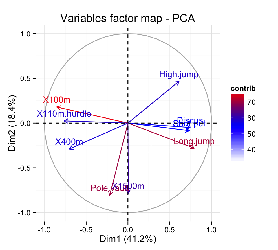
Contributions of the variables to the principal components
The contribution of a variable to a given principal component is (in percentage) : (var.cos2 * 100) / (total cos2 of the component)
comp.cos2 <- apply(var.cos2, 2, sum)

contrib <- function(var.cos2, comp.cos2){var.cos2*100/comp.cos2}

var.contrib <- t(apply(var.cos2,1, contrib, comp.cos2))
head(var.contrib[, 1:4])
PC1 PC2 PC3 PC4
X100m 17.544293 1.7505098 7.338659 0.13755240
Long.jump 15.293168 4.2904162 2.930094 1.62485936
Shot.put 13.060137 0.3967224 21.620432 2.01407269
High.jump 9.024811 11.7715838 8.792888 2.54987951
X400m 11.935544 4.5799296 6.487636 22.65090599
X110m.hurdle 14.157544 0.0332933 16.261261 0.03483735Highlight the most important (i.e, contributing) variables :
fviz_pca_var(res.pca, col.var="contrib") +
scale_color_gradient2(low="white", mid="blue",
      high="red", midpoint=50) + theme_minimal()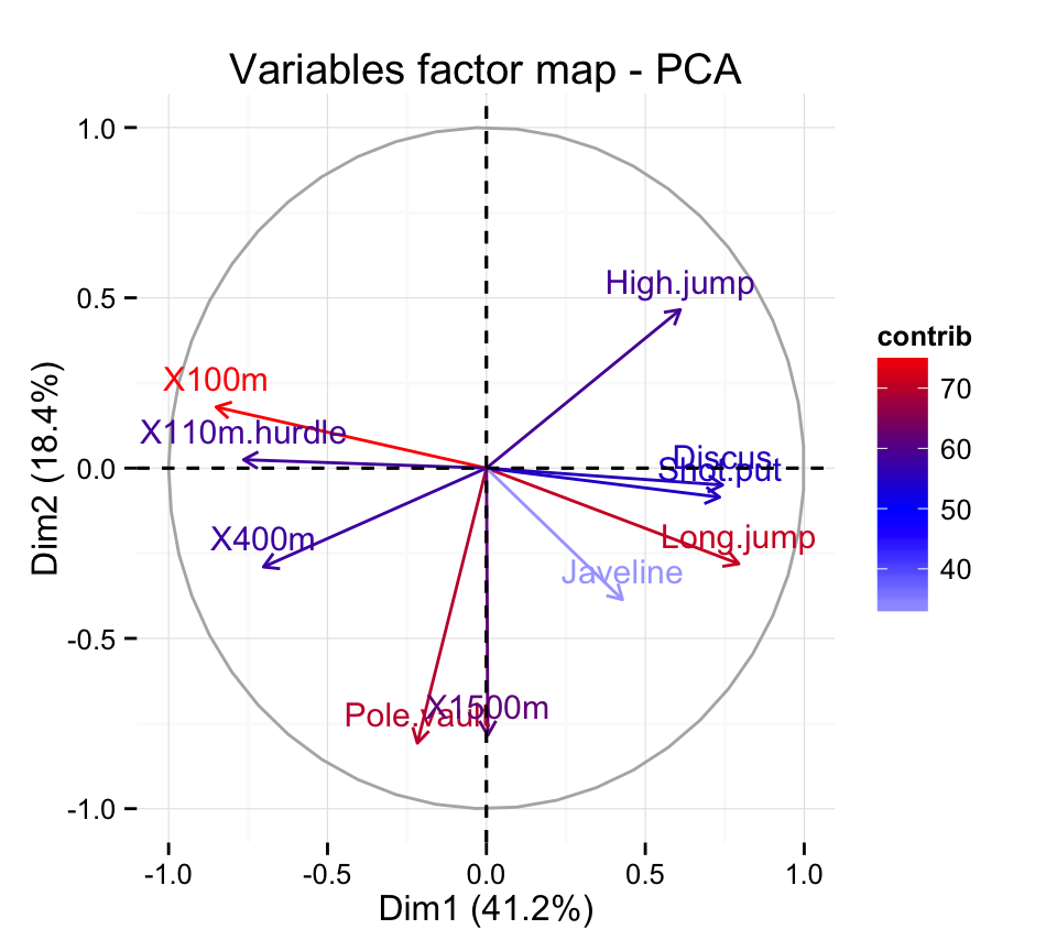
You can also use the function fviz_contrib() described here : Principal Component Analysis: How to reveal the most important variables in your data?
Graph of individuals
Coordinates of individuals on the principal components
ind.coord <- res.pca$x
head(ind.coord[, 1:4])
PC1 PC2 PC3 PC4
SEBRLE 0.1912074 -1.5541282 -0.6283688 0.08205241
CLAY 0.7901217 -2.4204156 1.3568870 1.26984296
BERNARD -1.3292592 -1.6118687 -0.1961500 -1.92092203
YURKOV -0.8694134 0.4328779 -2.4739822 0.69723814
ZSIVOCZKY -0.1057450 2.0233632 1.3049312 -0.09929630
McMULLEN 0.1185550 0.9916237 0.8435582 1.31215266Cos2 : quality of representation for individuals on the principal components
To calculate the cos2 of individuals, 2 simple steps are required :
- Calculate the square distance between each individual and the PCA center of gravity
- d2 = [(var1_ind_i - mean_var1)/sd_var1]^2 + + [(var10_ind_i - mean_var10)/sd_var10]^2 + +..
- Calculate the cos2 = ind.coord^2/d2
# Compute the square of the distance between an individual and the
# center of gravity
center <- res.pca$center
scale<- res.pca$scale
getdistance <- function(ind_row, center, scale){
  return(sum(((ind_row-center)/scale)^2))
  }
d2 <- apply(decathlon2.active,1,getdistance, center, scale)

# Compute the cos2
cos2 <- function(ind.coord, d2){return(ind.coord^2/d2)}
ind.cos2 <- apply(ind.coord, 2, cos2, d2)
head(ind.cos2[, 1:4])
PC1 PC2 PC3 PC4
SEBRLE 0.007530179 0.49747323 0.081325232 0.001386688
CLAY 0.048701249 0.45701660 0.143628117 0.125791741
BERNARD 0.197199804 0.28996555 0.004294015 0.411819183
YURKOV 0.096109800 0.02382571 0.778230322 0.061812637
ZSIVOCZKY 0.001574385 0.57641944 0.239754152 0.001388216
McMULLEN 0.002175437 0.15219499 0.110137872 0.266486530The sum of each row is 1, if we consider the 10 components
Contribution of individuals to the princial components
The contribution of individuals (in percentage) to the principal components can be computed as follow :
100 * (1 / number_of_individuals)*(ind.coord^2 / comp_sdev^2)
# Contributions of individuals
contrib <- function(ind.coord, comp.sdev, n.ind){
  100*(1/n.ind)*ind.coord^2/comp.sdev^2
}

ind.contrib <- t(apply(ind.coord,1, contrib,
                       res.pca$sdev, nrow(ind.coord)))
head(ind.contrib[, 1:4])
PC1 PC2 PC3 PC4
SEBRLE 0.03854254 5.7118249 1.3854184 0.03572215
CLAY 0.65814114 13.8541889 6.4600973 8.55568792
BERNARD 1.86273218 6.1441319 0.1349983 19.57827284
YURKOV 0.79686310 0.4431309 21.4755770 2.57939100
ZSIVOCZKY 0.01178829 9.6816398 5.9748485 0.05231437
McMULLEN 0.01481737 2.3253860 2.4967890 9.13531719Note that the sum of all the contributions per column is 100
Graph of individuals : base graph
plot(ind.coord[,1], ind.coord[,2], pch = 19,
     xlab="PC1 - 41.2%",ylab="PC2 - 18.4%")
abline(h=0, v=0, lty = 2)
text(ind.coord[,1], ind.coord[,2], labels=rownames(ind.coord),
        cex=0.7, pos = 3)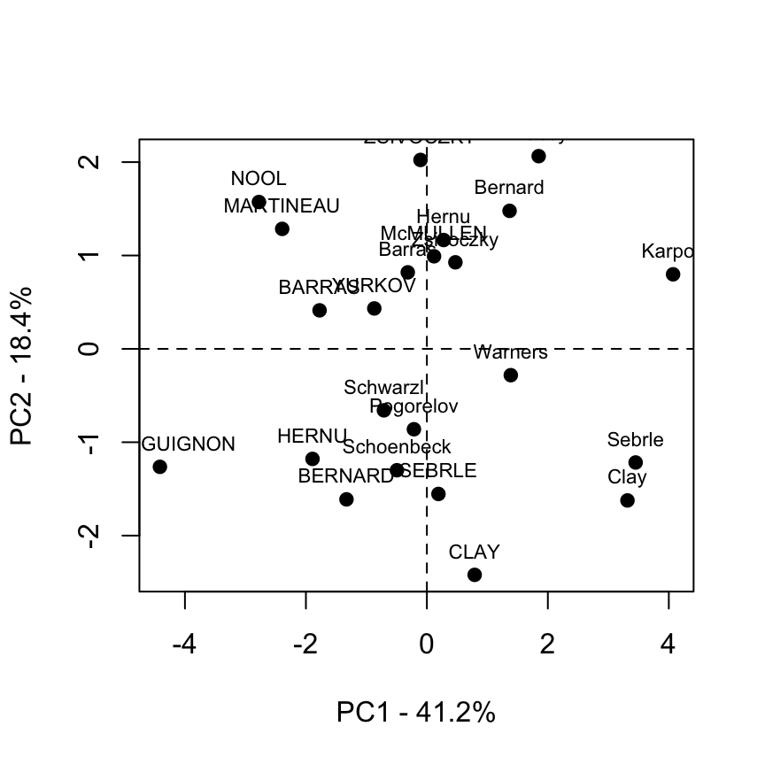
Biplot of individuals and variables :
biplot(res.pca, cex = 0.8, col = c("black", "red") )
Graph of individuals : factoextra
Extract the results for the individuals
factoextra provides, with less code, a list of matrices containing all the results for the active individuals (coordinates, square cosine, contributions).
ind <- get_pca_ind(res.pca)
ind
Principal Component Analysis Results for individuals
===================================================
Name Description
1 "$coord" "Coordinates for the individuals"
2 "$cos2" "Cos2 for the individuals"
3 "$contrib" "contributions of the individuals"# Coordinates for individuals
head(ind$coord[, 1:4]) Dim.1 Dim.2 Dim.3 Dim.4
SEBRLE 0.1912074 -1.5541282 -0.6283688 0.08205241
CLAY 0.7901217 -2.4204156 1.3568870 1.26984296
BERNARD -1.3292592 -1.6118687 -0.1961500 -1.92092203
YURKOV -0.8694134 0.4328779 -2.4739822 0.69723814
ZSIVOCZKY -0.1057450 2.0233632 1.3049312 -0.09929630
McMULLEN 0.1185550 0.9916237 0.8435582 1.31215266Graph of individuals using factoextra
Note that, in the R code below, the argument data is required only when res.pca is an object of class princomp or prcomp (two functions from the built-in Rstats package).
In other words, if res.pca is a result of PCA functions from FactoMineR or ade4 package, the argument data can be omitted.
Yes, factoextra can also handle the output of FactoMineR and ade4 packages.Default individuals factor map :
fviz_pca_ind(res.pca)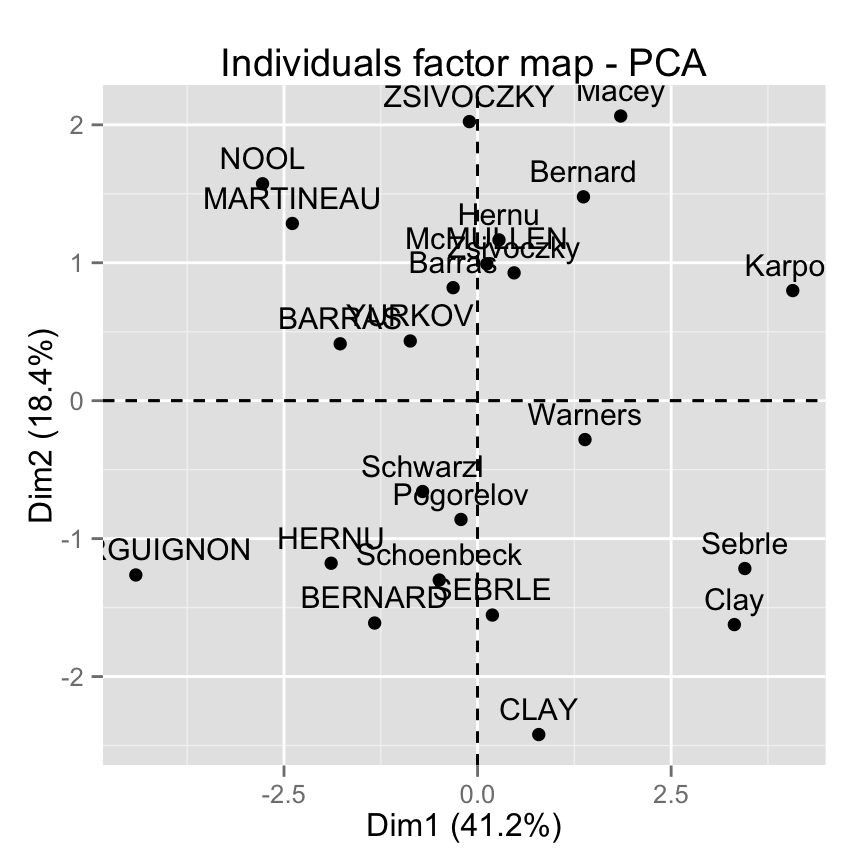
Control automatically the color of individuals using the cos2 values (the quality of the individuals on the factor map) :
fviz_pca_ind(res.pca, col.ind="cos2") +
scale_color_gradient2(low="white", mid="blue",
    high="red", midpoint=0.50) + theme_minimal()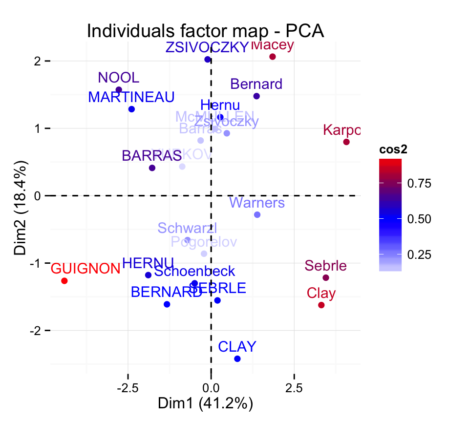
Read more about fviz_pca_ind() : Graph of individuals - principal component analysis
Make a biplot of individuals and variables :
fviz_pca_biplot(res.pca,  geom = "text") +
  theme_minimal()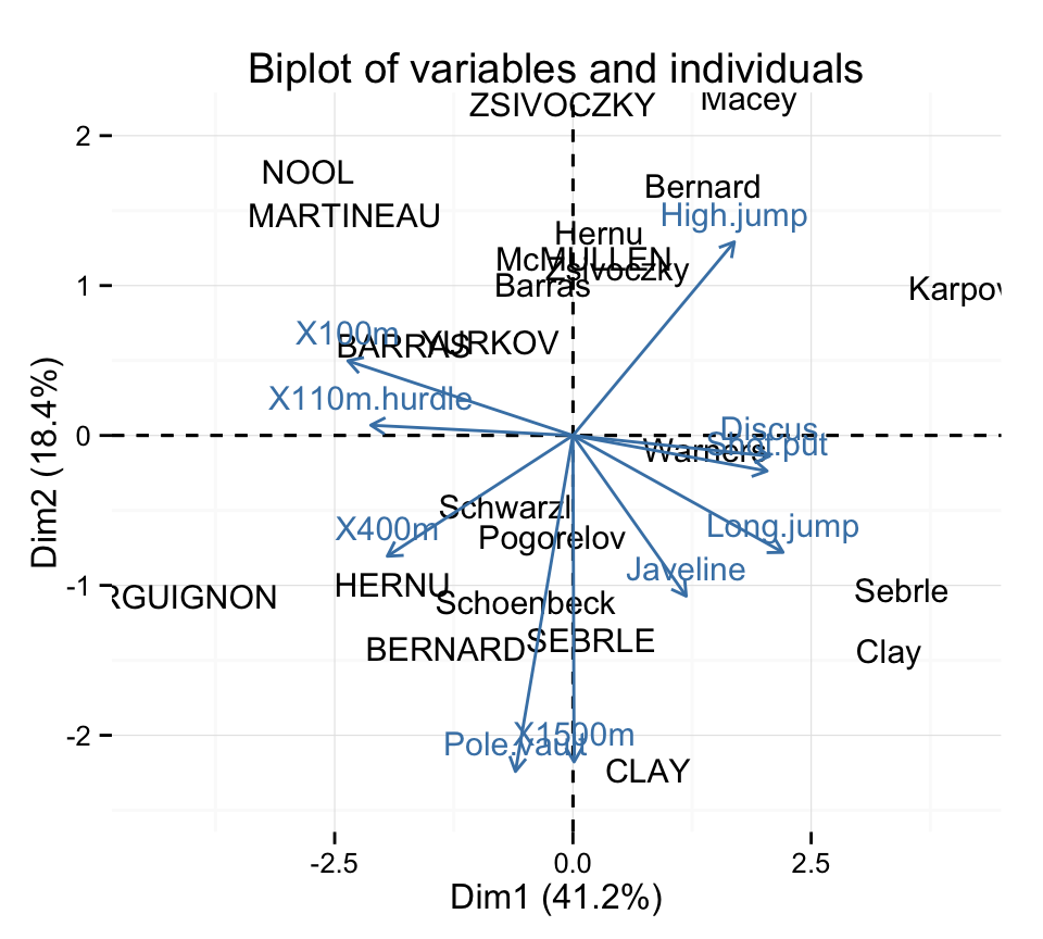
Read more about fviz_pca_biplot() : Biplot of individuals and variables - principal component analysis
Prediction using Principal Component Analysis
Supplementary quantitative variables
As described above, the data sets decathlon2 contain some supplementary continuous variables at columns 11 and 12 corresponding respectively to the rank and the points of athletes.
# Data for the supplementary quantitative variables
quanti.sup <- decathlon2[1:23, 11:12, drop = FALSE]
head(quanti.sup)
Rank Points
SEBRLE 1 8217
CLAY 2 8122
BERNARD 4 8067
YURKOV 5 8036
ZSIVOCZKY 7 8004
McMULLEN 8 7995Recall that, rows 24:27 are supplementary individuals. We dont want them in this current analysis. This is why, I extracted only rows 1:23.
In this section well see how to calculate the predicted coordinates of these two variables using the information provided by the previously performed principal component analysis.
2 simples steps are required :
- Calculate the correlation between each supplementary quantitative variables and the principal components
- Make a factor map of all variables (active and supplementary ones) to visualize the position of the supplementary variables
The R code below can be used :
# Calculate the correlations between supplementary variables
# and the principal components
ind.coord <- res.pca$x
quanti.coord <- cor(quanti.sup, ind.coord)
head(quanti.coord[, 1:4])
PC1 PC2 PC3 PC4
Rank -0.7014777 0.24519443 0.1834294 0.05575186
Points 0.9637075 -0.07768262 -0.1580225 -0.16623092# Variable factor maps
#++++++++++++++++++
# Plot the correlation circle
a <- seq(0, 2*pi, length = 100)
plot( cos(a), sin(a), type = 'l', col="gray",
xlab = "PC1", ylab = "PC2")
abline(h = 0, v = 0, lty = 2)
# Add active variables
var.coord <- get_pca_var(res.pca)$coord
arrows(0 ,0, x1=var.coord[,1], y1 = var.coord[,2],
col="black", length = 0.09)
text(var.coord[,1], var.coord[,2],
labels=rownames(var.coord), cex=0.8)
# Add supplementary quantitative variables
arrows(0 ,0, x1= quanti.coord[,1], y1 = quanti.coord[,2],
col="blue", lty =2, length = 0.09)
text(quanti.coord[,1], quanti.coord[,2],
labels=rownames(quanti.coord), cex=0.8, col ="blue")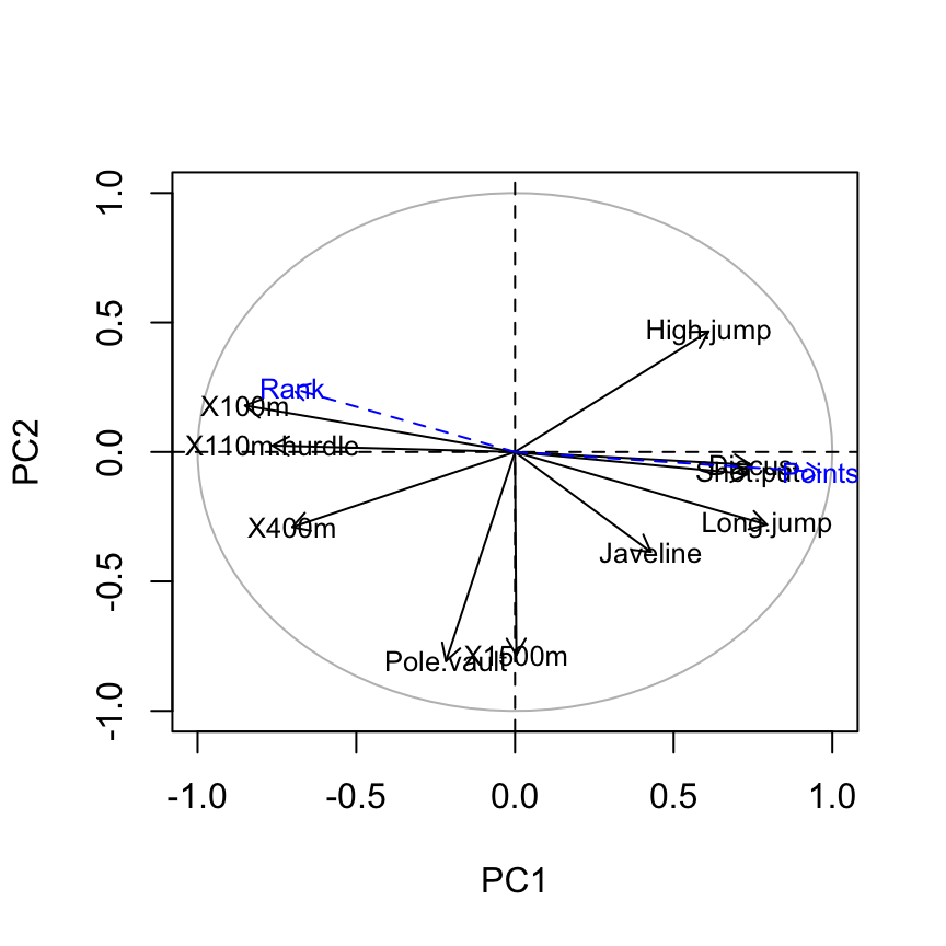
Its also possible to make the graph of variables using factoextra:
# Plot of active variables
p <- fviz_pca_var(res.pca)
# Add supplementary active variables
fviz_add(p, quanti.coord, color ="blue", geom="arrow")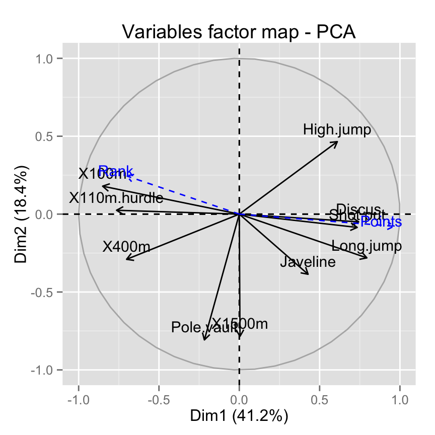
# get the cos2 of the supplementary quantitative variables
(quanti.coord^2)[, 1:4]
PC1 PC2 PC3 PC4
Rank 0.4920710 0.060120310 0.03364635 0.00310827
Points 0.9287322 0.006034589 0.02497110 0.02763272Supplementary qualitative variables
The data sets decathlon2 contain a supplementary qualitative variable at columns 13 corresponding to the type of competitions.
Qualitative variable can be helpful for interpreting the data and for coloring individuals by groups :
# Data for the supplementary qualitative variables
quali.sup <- as.factor(decathlon2[1:23, 13])
head(quali.sup)
[1] Decastar Decastar Decastar Decastar Decastar Decastar
Levels: Decastar OlympicGColor individuals by groups :
fviz_pca_ind(res.pca,
  habillage = quali.sup, addEllipses = TRUE, ellipse.level = 0.68) +
  theme_minimal()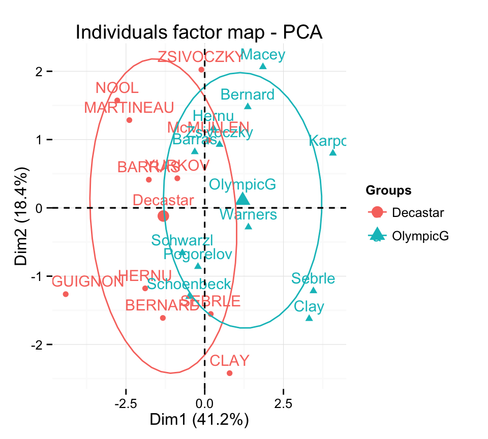
Note that, the argument habillage is used to specify the variable containing the groups of individuals
Its very easy to get the coordinates for the levels of a supplementary qualitative variables. The helper function below can be used :
# Return the coordinates of a group levels
# x : coordinate of individuals on x axis
# y : coordinate of indiviuals on y axis
get_coord_quali<-function(x, y, groups){
  data.frame(
    x= tapply(x, groups, mean),
    y = tapply(y, groups, mean)
  )
}
Calculate the coordinates on components 1 and 2 :
coord.quali <- get_coord_quali(ind.coord[,1], ind.coord[,2],
                               groups = quali.sup)
coord.quali
x y
Decastar -1.313921 -0.1191322
OlympicG 1.204428 0.1092046Supplementary individuals
The data sets decathlon2 contain some supplementary individuals from row 24 to 27.
# Data for the supplementary individuals
ind.sup <- decathlon2[24:27, 1:10, drop = FALSE]
ind.sup[, 1:6]
X100m Long.jump Shot.put High.jump X400m X110m.hurdle
KARPOV 11.02 7.30 14.77 2.04 48.37 14.09
WARNERS 11.11 7.60 14.31 1.98 48.68 14.23
Nool 10.80 7.53 14.26 1.88 48.81 14.80
Drews 10.87 7.38 13.07 1.88 48.51 14.01Remember that, columns 11:13 are supplementary variables. We dont want them in this current analysis. This is why, I extracted only columns 1:10. I used also the argument drop = FALSE to preserve the type of the data (which is a data.frame).
In this section well see how to predict the coordinates of the supplementary individuals using only the information provided by the previously performed principal component analysis.
A simple function to predict the coordinates of new individuals data
One simple approach is to use the function predict() from the built-in R stats package :
ind.sup.coord <- predict(res.pca, newdata = ind.sup)
ind.sup.coord[, 1:4]
PC1 PC2 PC3 PC4
KARPOV 0.7772521 -0.76237804 1.5971253 1.6863286
WARNERS -0.3779697 0.11891968 1.7005146 -0.6908084
Nool -0.5468405 -1.93402211 0.4724184 -2.2283706
Drews -1.0848227 -0.01703198 2.9818031 -1.5006207Calculate the predicted coordinates by hand
2 simples steps are required :
- Center and scale the values for the supplementary individuals using the center and the scale of the PCA
- Calculate the predicted coordinates by multiplying the scaled values with the eigenvectors (loadings) of the principal components.
The R code below can be used :
# Centering and scaling the supplementary individuals
scale_func <- function(ind_row, center, scale){
  (ind_row-center)/scale
}

ind.scaled <- t(apply(ind.sup, 1, scale_func, res.pca$center, res.pca$scale))

# Coordinates of the individividuals
pca.loadings <- res.pca$rotation
coord_func <- function(ind, loadings){
  r <- loadings*ind
  r <- apply(r, 2, sum)
  r
}

ind.sup.coord <- t(apply(ind.scaled, 1, coord_func, pca.loadings ))
ind.sup.coord[, 1:4]
PC1 PC2 PC3 PC4
KARPOV 0.7772521 -0.76237804 1.5971253 1.6863286
WARNERS -0.3779697 0.11891968 1.7005146 -0.6908084
Nool -0.5468405 -1.93402211 0.4724184 -2.2283706
Drews -1.0848227 -0.01703198 2.9818031 -1.5006207Make a factor map including the supplementary individuals using factoextra
# Plot of active individuals
p <- fviz_pca_ind(res.pca)
# Add supplementary individuals
fviz_add(p, ind.sup.coord, color ="blue")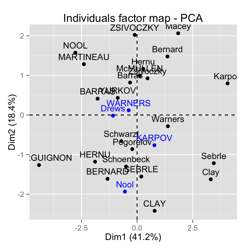
Infos
This analysis has been performed using R software (ver. 3.1.2) and factoextra (ver. 1.0.2)
Read more :
- Gregory B. Anderson, principal component analysis in R, https://www.ime.usp.br/~pavan/pdf/MAE0330-PCA-R-2013
