Survival Analysis Basics

Survival time and type of events in cancer studies

There are different types of events, including:

• Relapse
• Progression
• Death

The time from ‘response to treatment’ (complete remission) to the occurrence of the event of interest is commonly called survival time (or time to event).

The two most important measures in cancer studies include: i) the time to death; and ii) the relapse-free survival time, which corresponds to the time between response to treatment and recurrence of the disease. It’s also known as disease-free survival time and event-free survival time.

Censoring

As mentioned above, survival analysis focuses on the expected duration of time until occurrence of an event of interest (relapse or death). However, the event may not be observed for some individuals within the study time period, producing the so-called censored observations.

Censoring may arise in the following ways:

1. a patient has not (yet) experienced the event of interest, such as relapse or death, within the study time period;
2. a patient is lost to follow-up during the study period;
3. a patient experiences a different event that makes further follow-up impossible.

This type of censoring, named right censoring, is handled in survival analysis.

Survival and hazard functions

Two related probabilities are used to describe survival data: the survival probability and the hazard probability.

The survival probability, also known as the survivor function \(S(t)\), is the probability that an individual survives from the time origin (e.g. diagnosis of cancer) to a specified future time t.

The hazard, denoted by \(h(t)\), is the probability that an individual who is under observation at a time t has an event at that time.

Note that, in contrast to the survivor function, which focuses on not having an event, the hazard function focuses on the event occurring.

Kaplan-Meier survival estimate

The Kaplan-Meier (KM) method is a non-parametric method used to estimate the survival probability from observed survival times (Kaplan and Meier, 1958).

The survival probability at time \(t_i\), \(S(t_i)\), is calculated as follow:

\[S(t_i) = S(t_{i-1})(1-\frac{d_i}{n_i})\]

Where,

• \(S(t_{i-1})\) = the probability of being alive at \(t_{i-1}\)
• \(n_i\) = the number of patients alive just before \(t_i\)
• \(d_i\) = the number of events at \(t_i\)
• \(t_0\) = 0, \(S(0)\) = 1

The estimated probability (\(S(t)\)) is a step function that changes value only at the time of each event. It’s also possible to compute confidence intervals for the survival probability.

The KM survival curve, a plot of the KM survival probability against time, provides a useful summary of the data that can be used to estimate measures such as median survival time.

Install and load required R package

We’ll use two R packages:

• survival for computing survival analyses

• survminer for summarizing and visualizing the results of survival analysis

• Install the packages

install.packages(c("survival", "survminer"))

• Load the packages

library("survival")
library("survminer")

Example data sets

We’ll use the lung cancer data available in the survival package.

data("lung")
head(lung)

  inst time status age sex ph.ecog ph.karno pat.karno meal.cal wt.loss
1    3  306      2  74   1       1       90       100     1175      NA
2    3  455      2  68   1       0       90        90     1225      15
3    3 1010      1  56   1       0       90        90       NA      15
4    5  210      2  57   1       1       90        60     1150      11
5    1  883      2  60   1       0      100        90       NA       0
6   12 1022      1  74   1       1       50        80      513       0

• inst: Institution code
• time: Survival time in days
• status: censoring status 1=censored, 2=dead
• age: Age in years
• sex: Male=1 Female=2
• ph.ecog: ECOG performance score (0=good 5=dead)
• ph.karno: Karnofsky performance score (bad=0-good=100) rated by physician
• pat.karno: Karnofsky performance score as rated by patient
• meal.cal: Calories consumed at meals
• wt.loss: Weight loss in last six months

Compute survival curves: survfit()

We want to compute the survival probability by sex.

The function survfit() [in survival package] can be used to compute kaplan-Meier survival estimate. Its main arguments include:

• a survival object created using the function Surv()
• and the data set containing the variables.

To compute survival curves, type this:

fit <- survfit(Surv(time, status) ~ sex, data = lung)
print(fit)

Call: survfit(formula = Surv(time, status) ~ sex, data = lung)

        n events median 0.95LCL 0.95UCL
sex=1 138    112    270     212     310
sex=2  90     53    426     348     550

By default, the function print() shows a short summary of the survival curves. It prints the number of observations, number of events, the median survival and the confidence limits for the median.

If you want to display a more complete summary of the survival curves, type this:

# Summary of survival curves
summary(fit)

# Access to the sort summary table
summary(fit)$table

Access to the value returned by survfit()

The function survfit() returns a list of variables, including the following components:

The components can be accessed as follow:

d <- data.frame(time = fit$time,
                  n.risk = fit$n.risk,
                  n.event = fit$n.event,
                  n.censor = fit$n.censor,
                  surv = fit$surv,
                  upper = fit$upper,
                  lower = fit$lower
                  )
head(d)

  time n.risk n.event n.censor      surv     upper     lower
1   11    138       3        0 0.9782609 1.0000000 0.9542301
2   12    135       1        0 0.9710145 0.9994124 0.9434235
3   13    134       2        0 0.9565217 0.9911586 0.9230952
4   15    132       1        0 0.9492754 0.9866017 0.9133612
5   26    131       1        0 0.9420290 0.9818365 0.9038355
6   30    130       1        0 0.9347826 0.9768989 0.8944820

Visualize survival curves

We’ll use the function ggsurvplot() [in Survminer R package] to produce the survival curves for the two groups of subjects.

It’s also possible to show:

• the 95% confidence limits of the survivor function using the argument conf.int = TRUE.
• the number and/or the percentage of individuals at risk by time using the option risk.table. Allowed values for risk.table include:
  • TRUE or FALSE specifying whether to show or not the risk table. Default is FALSE.
  • “absolute” or “percentage”: to show the absolute number and the percentage of subjects at risk by time, respectively. Use “abs_pct” to show both absolute number and percentage.
• the p-value of the Log-Rank test comparing the groups using pval = TRUE.
• horizontal/vertical line at median survival using the argument surv.median.line. Allowed values include one of c(“none”, “hv”, “h”, “v”). v: vertical, h:horizontal.

# Change color, linetype by strata, risk.table color by strata
ggsurvplot(fit,
          pval = TRUE, conf.int = TRUE,
          risk.table = TRUE, # Add risk table
          risk.table.col = "strata", # Change risk table color by groups
          linetype = "strata", # Change line type by groups
          surv.median.line = "hv", # Specify median survival
          ggtheme = theme_bw(), # Change ggplot2 theme
          palette = c("#E7B800", "#2E9FDF"))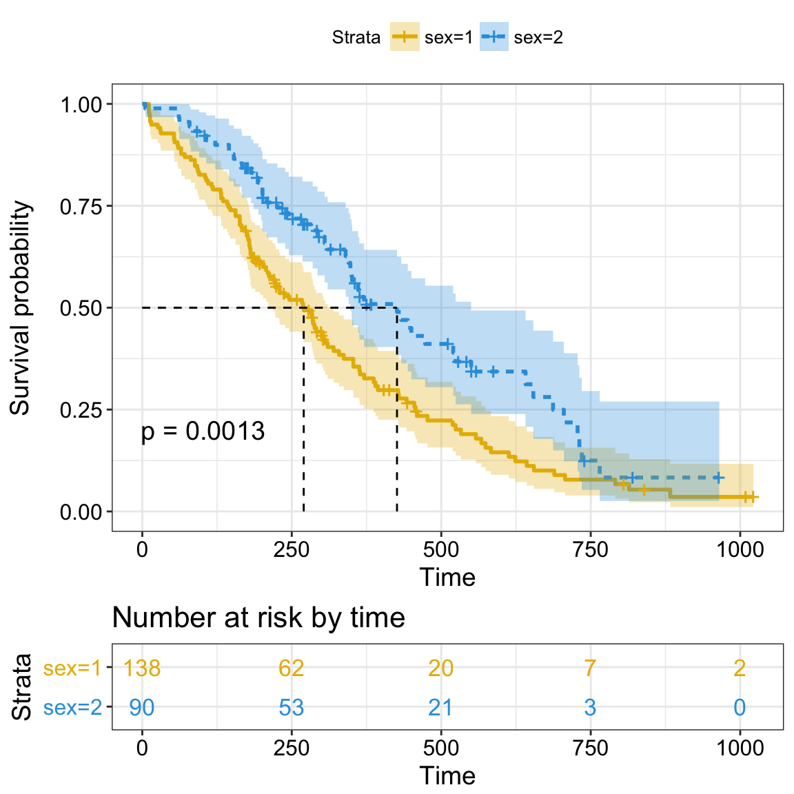

Survival Analysis

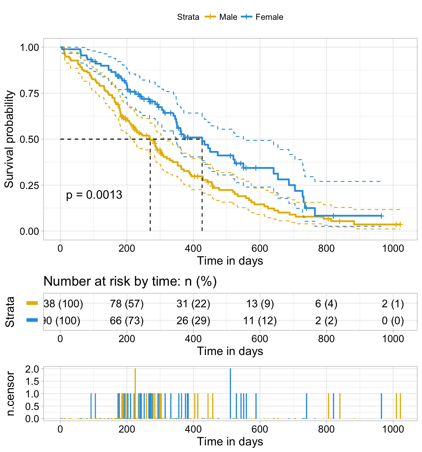
The plot can be further customized using the following arguments:

• conf.int.style = “step” to change the style of confidence interval bands.
• xlab to change the x axis label.
• break.time.by = 200 break x axis in time intervals by 200.
• risk.table = “abs_pct”to show both absolute number and percentage of individuals at risk.
• risk.table.y.text.col = TRUE and risk.table.y.text = FALSE to provide bars instead of names in text annotations of the legend of risk table.
• ncensor.plot = TRUE to plot the number of censored subjects at time t. As suggested by Marcin Kosinski, This is a good additional feedback to survival curves, so that one could realize: how do survival curves look like, what is the number of risk set AND what is the cause that the risk set become smaller: is it caused by events or by censored events?
• legend.labs to change the legend labels.

ggsurvplot(
   fit,                     # survfit object with calculated statistics.
   pval = TRUE,             # show p-value of log-rank test.
   conf.int = TRUE,         # show confidence intervals for 
                            # point estimaes of survival curves.
   conf.int.style = "step",  # customize style of confidence intervals
   xlab = "Time in days",   # customize X axis label.
   break.time.by = 200,     # break X axis in time intervals by 200.
   ggtheme = theme_light(), # customize plot and risk table with a theme.
   risk.table = "abs_pct",  # absolute number and percentage at risk.
  risk.table.y.text.col = T,# colour risk table text annotations.
  risk.table.y.text = FALSE,# show bars instead of names in text annotations
                            # in legend of risk table.
  ncensor.plot = TRUE,      # plot the number of censored subjects at time t
  surv.median.line = "hv",  # add the median survival pointer.
  legend.labs = 
    c("Male", "Female"),    # change legend labels.
  palette = 
    c("#E7B800", "#2E9FDF") # custom color palettes.
)

Survival Analysis

The Kaplan-Meier plot can be interpreted as follow:

The median survival times for each group can be obtained using the code below:

summary(fit)$table

      records n.max n.start events   *rmean *se(rmean) median 0.95LCL 0.95UCL
sex=1     138   138     138    112 325.0663   22.59845    270     212     310
sex=2      90    90      90     53 458.2757   33.78530    426     348     550

The median survival times for each group represent the time at which the survival probability, S(t), is 0.5.

The median survival time for sex=1 (Male group) is 270 days, as opposed to 426 days for sex=2 (Female). There appears to be a survival advantage for female with lung cancer compare to male. However, to evaluate whether this difference is statistically significant requires a formal statistical test, a subject that is discussed in the next sections.

Note that, the confidence limits are wide at the tail of the curves, making meaningful interpretations difficult. This can be explained by the fact that, in practice, there are usually patients who are lost to follow-up or alive at the end of follow-up. Thus, it may be sensible to shorten plots before the end of follow-up on the x-axis (Pocock et al, 2002).

The survival curves can be shorten using the argument xlim as follow:

ggsurvplot(fit,
          conf.int = TRUE,
          risk.table.col = "strata", # Change risk table color by groups
          ggtheme = theme_bw(), # Change ggplot2 theme
          palette = c("#E7B800", "#2E9FDF"),
          xlim = c(0, 600))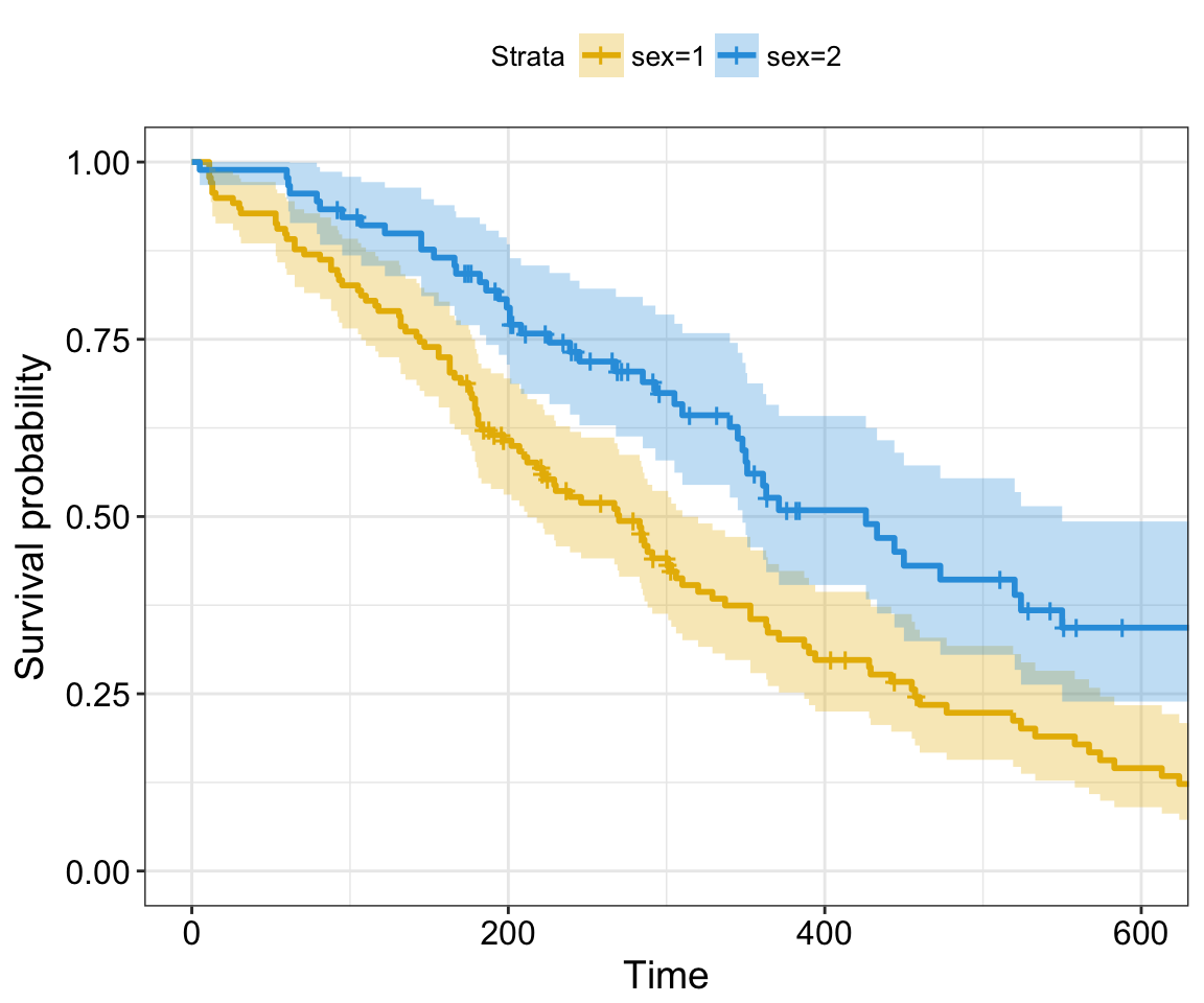

Survival Analysis

For example, to plot cumulative events, type this:

ggsurvplot(fit,
          conf.int = TRUE,
          risk.table.col = "strata", # Change risk table color by groups
          ggtheme = theme_bw(), # Change ggplot2 theme
          palette = c("#E7B800", "#2E9FDF"),
          fun = "event")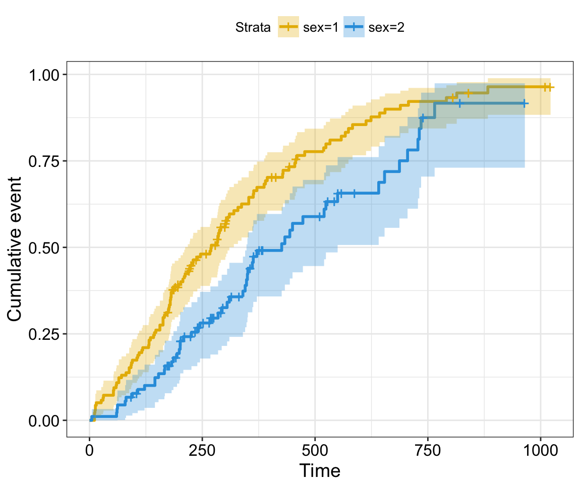

Survival Analysis

The cummulative hazard is commonly used to estimate the hazard probability. It’s defined as \(H(t) = -log(survival function) = -log(S(t))\). The cumulative hazard (\(H(t)\)) can be interpreted as the cumulative force of mortality. In other words, it corresponds to the number of events that would be expected for each individual by time t if the event were a repeatable process.

To plot cumulative hazard, type this:

ggsurvplot(fit,
          conf.int = TRUE,
          risk.table.col = "strata", # Change risk table color by groups
          ggtheme = theme_bw(), # Change ggplot2 theme
          palette = c("#E7B800", "#2E9FDF"),
          fun = "cumhaz")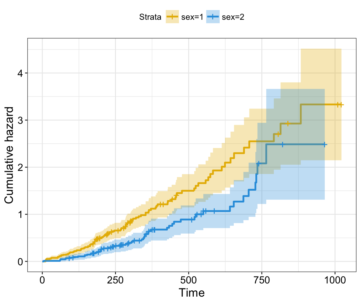

Survival Analysis

Kaplan-Meier life table: summary of survival curves

As mentioned above, you can use the function summary() to have a complete summary of survival curves:

summary(fit)

It’s also possible to use the function surv_summary() [in survminer package] to get a summary of survival curves. Compared to the default summary() function, surv_summary() creates a data frame containing a nice summary from survfit results.

res.sum <- surv_summary(fit)
head(res.sum)

  time n.risk n.event n.censor      surv    std.err     upper     lower strata sex
1   11    138       3        0 0.9782609 0.01268978 1.0000000 0.9542301  sex=1   1
2   12    135       1        0 0.9710145 0.01470747 0.9994124 0.9434235  sex=1   1
3   13    134       2        0 0.9565217 0.01814885 0.9911586 0.9230952  sex=1   1
4   15    132       1        0 0.9492754 0.01967768 0.9866017 0.9133612  sex=1   1
5   26    131       1        0 0.9420290 0.02111708 0.9818365 0.9038355  sex=1   1
6   30    130       1        0 0.9347826 0.02248469 0.9768989 0.8944820  sex=1   1

The function surv_summary() returns a data frame with the following columns:

• time: the time points at which the curve has a step.
• n.risk: the number of subjects at risk at t.
• n.event: the number of events that occur at time t.
• n.censor: number of censored events.
• surv: estimate of survival probability.
• std.err: standard error of survival.
• upper: upper end of confidence interval
• lower: lower end of confidence interval
• strata: indicates stratification of curve estimation. The levels of strata (a factor) are the labels for the curves.

In a situation, where survival curves have been fitted with one or more variables, surv_summary object contains extra columns representing the variables. This makes it possible to facet the output of ggsurvplot by strata or by some combinations of factors.

surv_summary object has also an attribute named ‘table’ containing information about the survival curves, including medians of survival with confidence intervals, as well as, the total number of subjects and the number of event in each curve. To get access to the attribute ‘table’, type this:

attr(res.sum, "table")

Log-Rank test comparing survival curves: survdiff()

The log-rank test is the most widely used method of comparing two or more survival curves. The null hypothesis is that there is no difference in survival between the two groups. The log rank test is a non-parametric test, which makes no assumptions about the survival distributions. Essentially, the log rank test compares the observed number of events in each group to what would be expected if the null hypothesis were true (i.e., if the survival curves were identical). The log rank statistic is approximately distributed as a chi-square test statistic.

The function survdiff() [in survival package] can be used to compute log-rank test comparing two or more survival curves.

survdiff() can be used as follow:

surv_diff <- survdiff(Surv(time, status) ~ sex, data = lung)
surv_diff

Call:
survdiff(formula = Surv(time, status) ~ sex, data = lung)

        N Observed Expected (O-E)^2/E (O-E)^2/V
sex=1 138      112     91.6      4.55      10.3
sex=2  90       53     73.4      5.68      10.3

 Chisq= 10.3  on 1 degrees of freedom, p= 0.00131 

The function returns a list of components, including:

• n: the number of subjects in each group.
• obs: the weighted observed number of events in each group.
• exp: the weighted expected number of events in each group.
• chisq: the chisquare statistic for a test of equality.
• strata: optionally, the number of subjects contained in each stratum.

The log rank test for difference in survival gives a p-value of p = 0.0013, indicating that the sex groups differ significantly in survival.

Fit complex survival curves

In this section, we’ll compute survival curves using the combination of multiple factors. Next, we’ll facet the output of ggsurvplot() by a combination of factors

1. Fit (complex) survival curves using colon data sets

require("survival")
fit2 <- survfit( Surv(time, status) ~ sex + rx + adhere,
                data = colon )

2. Visualize the output using survminer. The plot below shows survival curves by the sex variable faceted according to the values of rx & adhere.

# Plot survival curves by sex and facet by rx and adhere
ggsurv <- ggsurvplot(fit2, fun = "event", conf.int = TRUE,
                     ggtheme = theme_bw())
   
ggsurv$plot +theme_bw() + 
  theme (legend.position = "right")+
  facet_grid(rx ~ adhere)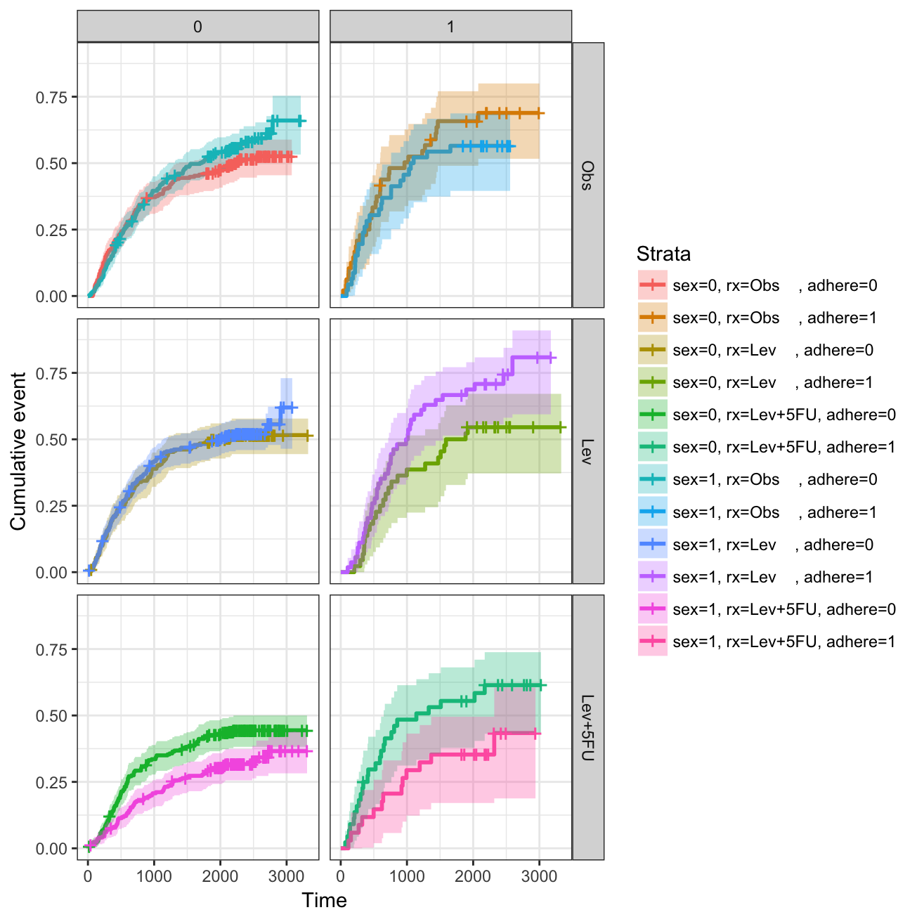

Survival Analysis

References

- Clark TG, Bradburn MJ, Love SB and Altman DG. Survival Analysis Part I: Basic concepts and first analyses. British Journal of Cancer (2003) 89, 232 – 238
- Kaplan EL, Meier P (1958) Nonparametric estimation from incomplete observations. J Am Stat Assoc 53: 457–481.
- Pocock S, Clayton TC, Altman DG (2002) Survival plots of time-to-event outcomes in clinical trials: good practice and pitfalls. Lancet 359: 1686– 1689.
Infos
This analysis has been performed using R software (ver. 3.3.2).