The first step in clustering analysis is to assess whether the dataset is clusterable. This has been described in a chapter entitled: Assessing Clustering Tendency.
Partitioning methods, such as k-means clustering require also the users to specify the number of clusters to be generated.
One fundamental question is: If the data is clusterable, then how to choose the right number of expected clusters (k)?
Unfortunately, there is no definitive answer to this question. The optimal clustering is somehow subjective and depend on the method used for measuring similarities and the parameters used for partitioning.
A simple and popular solution consists of inspecting the dendrogram produced using hierarchical clustering to see if it suggests a particular number of clusters. Unfortunately this approach is, again, subjective.
In this article, well describe different methods for determining the optimal number of clusters for k-means, PAM and hierarchical clustering . These methods include direct methods and statistical testing methods.
- Direct methods consists of optimizing a criterion, such as the within cluster sums of squares or the average silhouette. The corresponding methods are named elbow and silhouette methods, respectively.
- Testing methods consists of comparing evidence against null hypothesis. An example is the gap statistic.
In addition to elbow, silhouette and gap statistic methods, there are more than thirty other indices and methods that have been published for identifying the optimal number of clusters. Well provide R codes for computing all these 30 indices in order to decide the best number of clusters using the majority rule.
For each of these methods:
- Well describe the basic idea, the algorithm and the key mathematical concept
- Well provide easy-o-use R codes with many examples for determining the optimal number of clusters and visualizing the output
1 Required packages
The following package will be used:
- cluster for computing pam and for analyzing cluster silhouettes
- factoextra for visualizing clusters using ggplot2 plotting system
- NbClust for finding the optimal number of clusters
Install factoextra package as follow:
if(!require(devtools)) install.packages("devtools")
devtools::install_github("kassambara/factoextra")
The remaining packages can be installed using the code below:
pkgs <- c("cluster",  "NbClust")
install.packages(pkgs)
Load packages:
library(factoextra)
library(cluster)
library(NbClust)
2 Data preparation
The data set iris is used. We start by excluding the species column and scaling the data using the function scale():
# Load the data
data(iris)
head(iris)
## Sepal.Length Sepal.Width Petal.Length Petal.Width Species
## 1 5.1 3.5 1.4 0.2 setosa
## 2 4.9 3.0 1.4 0.2 setosa
## 3 4.7 3.2 1.3 0.2 setosa
## 4 4.6 3.1 1.5 0.2 setosa
## 5 5.0 3.6 1.4 0.2 setosa
## 6 5.4 3.9 1.7 0.4 setosa# Remove species column (5) and scale the data
iris.scaled <- scale(iris[, -5])This iris data set gives the measurements in centimeters of the variables sepal length and width and petal length and width, respectively, for 50 flowers from each of 3 species of iris. The species are Iris setosa, versicolor, and virginica.
3 Example of partitioning method results
The functions kmeans() [in stats package] and pam() [in cluster package] are described in this section. Well split the data into 3 clusters as follow:
# K-means clustering
set.seed(123)
km.res <- kmeans(iris.scaled, 3, nstart = 25)
# k-means group number of each observation
km.res$cluster
## [1] 1 1 1 1 1 1 1 1 1 1 1 1 1 1 1 1 1 1 1 1 1 1 1 1 1 1 1 1 1 1 1 1 1 1 1
## [36] 1 1 1 1 1 1 1 1 1 1 1 1 1 1 1 2 2 2 3 3 3 2 3 3 3 3 3 3 3 3 2 3 3 3 3
## [71] 2 3 3 3 3 2 2 2 3 3 3 3 3 3 3 2 2 3 3 3 3 3 3 3 3 3 3 3 3 3 2 3 2 2 2
## [106] 2 3 2 2 2 2 2 2 3 3 2 2 2 2 3 2 3 2 3 2 2 3 2 2 2 2 2 2 3 3 2 2 2 3 2
## [141] 2 2 3 2 2 2 3 2 2 3# Visualize k-means clusters
fviz_cluster(km.res, data = iris.scaled, geom = "point",
stand = FALSE, frame.type = "norm")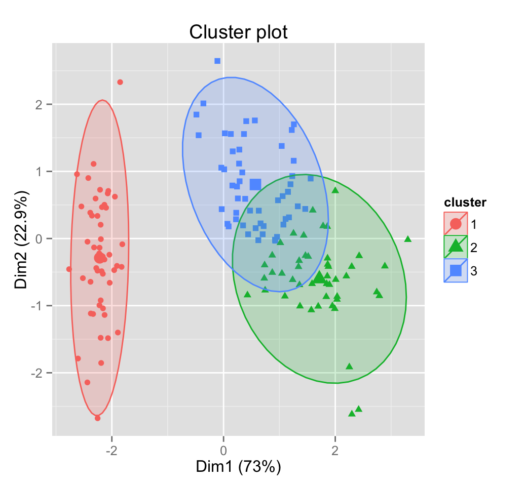
# PAM clustering
library("cluster")
pam.res <- pam(iris.scaled, 3)
pam.res$cluster
## [1] 1 1 1 1 1 1 1 1 1 1 1 1 1 1 1 1 1 1 1 1 1 1 1 1 1 1 1 1 1 1 1 1 1 1 1
## [36] 1 1 1 1 1 1 1 1 1 1 1 1 1 1 1 2 2 2 3 3 3 2 3 3 3 3 3 3 3 3 2 3 3 3 3
## [71] 3 3 3 3 3 2 2 2 3 3 3 3 3 3 3 3 2 3 3 3 3 3 3 3 3 3 3 3 3 3 2 3 2 2 2
## [106] 2 3 2 2 2 2 2 2 3 2 2 2 2 2 3 2 3 2 3 2 2 3 3 2 2 2 2 2 3 3 2 2 2 3 2
## [141] 2 2 3 2 2 2 3 2 2 3# Visualize pam clusters
fviz_cluster(pam.res, stand = FALSE, geom = "point",
frame.type = "norm")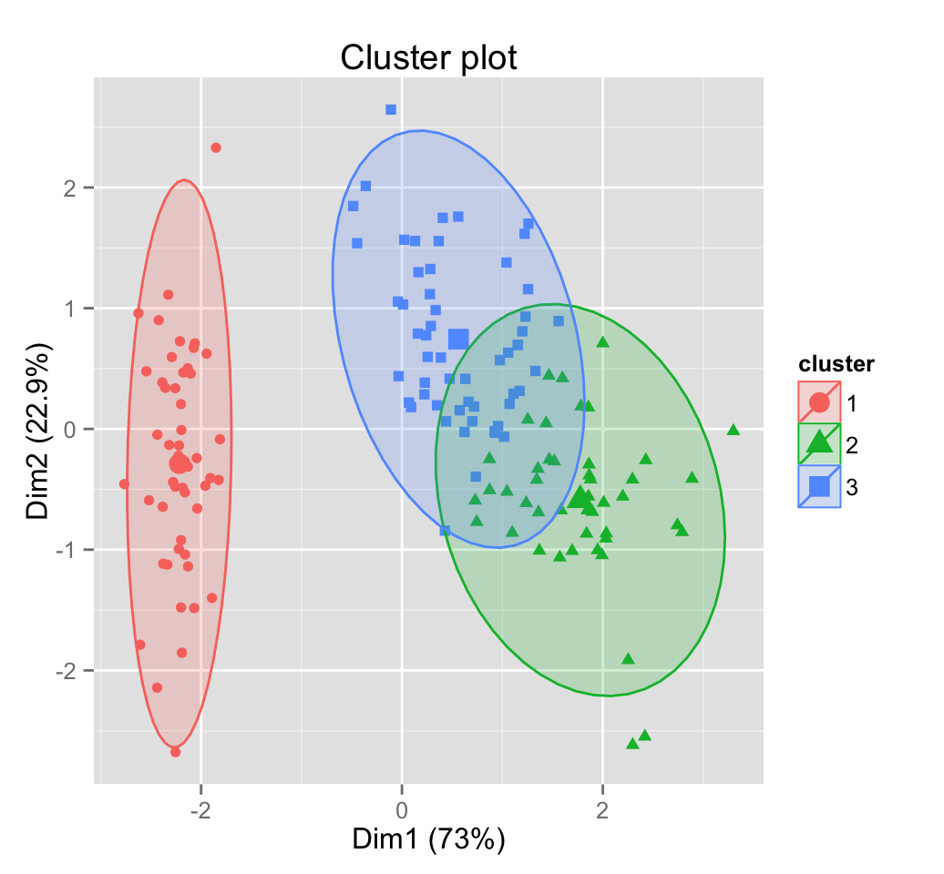
Read more about partitioning methods: Partitioning clustering
4 Example of hierarchical clustering results
The built-in R function hclust() is used:
# Compute pairewise distance matrices
dist.res <- dist(iris.scaled, method = "euclidean")
# Hierarchical clustering results
hc <- hclust(dist.res, method = "complete")
# Visualization of hclust
plot(hc, labels = FALSE, hang = -1)
# Add rectangle around 3 groups
rect.hclust(hc, k = 3, border = 2:4) 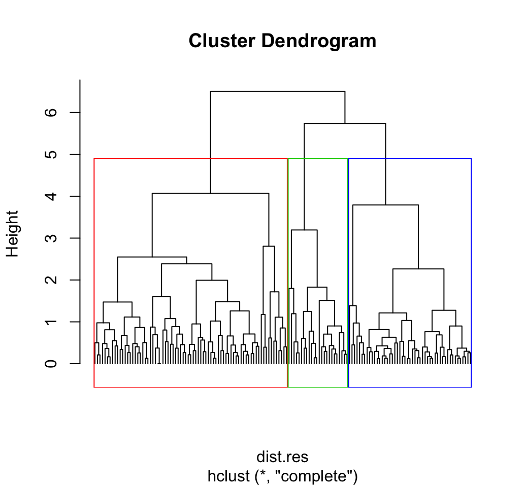
# Cut into 3 groups
hc.cut <- cutree(hc, k = 3)
head(hc.cut, 20)
## [1] 1 1 1 1 1 1 1 1 1 1 1 1 1 1 1 1 1 1 1 1Read more about hierarchical clustering: Hierarchical clustering
5 Three popular methods for determining the optimal number of clusters
In this section we describe the three most popular methods including: i) Elbow method, ii) silhouette method and iii) gap statistic.
5.1 Elbow method
5.1.1 Concept
Recall that, the basic idea behind partitioning methods, such as k-means clustering, is to define clusters such that the total intra-cluster variation (known as total within-cluster variation or total within-cluster sum of square) is minimized:
\(minimize\left(\sum\limits_{k=1}^k W(C_k)\right)\),
Where \(C_k\) is the \(k_{th}\) cluster and \(W(C_k)\) is the within-cluster variation.
The total within-cluster sum of square (wss) measures the compactness of the clustering and we want it to be as small as possible.
5.1.2 Algorithm
The optimal number of clusters can be defined as follow:
- Compute clustering algorithm (e.g., k-means clustering) for different values of k. For instance, by varying k from 1 to 10 clusters
- For each k, calculate the total within-cluster sum of square (wss)
- Plot the curve of wss according to the number of clusters k.
- The location of a bend (knee) in the plot is generally considered as an indicator of the appropriate number of clusters.
5.1.3 R codes
5.1.3.1 Elbow method for k-means clustering
set.seed(123)
# Compute and plot wss for k = 2 to k = 15
k.max <- 15 # Maximal number of clusters
data <- iris.scaled
wss <- sapply(1:k.max,
        function(k){kmeans(data, k, nstart=10 )$tot.withinss})

plot(1:k.max, wss,
       type="b", pch = 19, frame = FALSE,
       xlab="Number of clusters K",
       ylab="Total within-clusters sum of squares")
abline(v = 3, lty =2)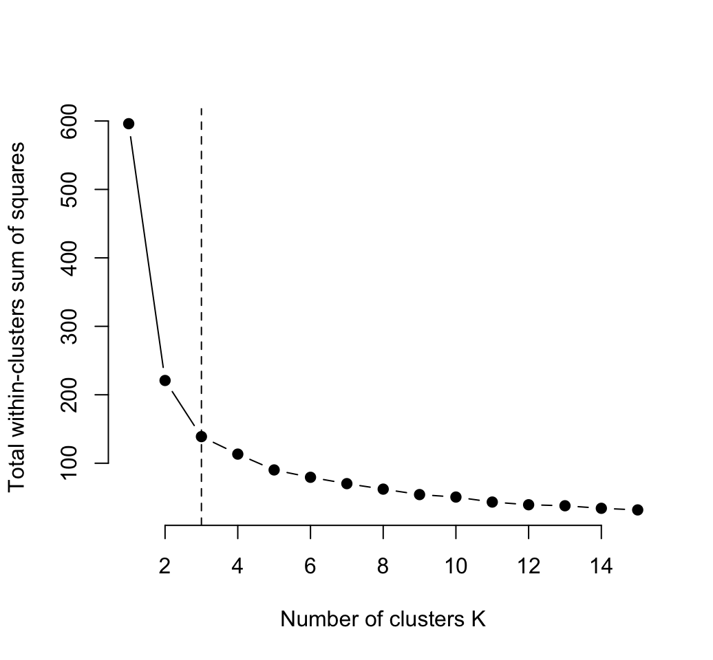
The elbow method suggests 3 cluster solutions.
The elbow method is implemented in factoextra package and can be easily computed using the function fviz_nbclust(), which format is:
fviz_nbclust(x, FUNcluster, method = c("silhouette", "wss"))- x: numeric matrix or data frame
- FUNcluster: a partitioning function such as kmeans, pam, clara etc
- method: the method to be used for determining the optimal number of clusters.
The R code below computes the elbow method for kmeans():
fviz_nbclust(iris.scaled, kmeans, method = "wss") +
    geom_vline(xintercept = 3, linetype = 2)
Three clusters are suggested.
5.1.3.2 Elbow method for PAM clustering
Its possible to use the function fviz_nbclust() as follow:
fviz_nbclust(iris.scaled, pam, method = "wss") +
  geom_vline(xintercept = 3, linetype = 2)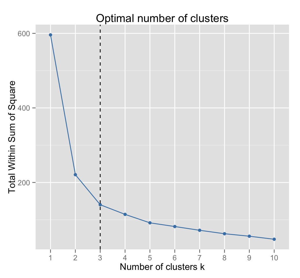
Three clusters are suggested.
5.1.3.3 Elbow method for hierarchical clustering
Well use a helper function hcut() [in factoextra package] which will compute hierarchical clustering (HC) algorithm and cut the dendrogram in k clusters:
fviz_nbclust(iris.scaled, hcut, method = "wss") +
  geom_vline(xintercept = 3, linetype = 2)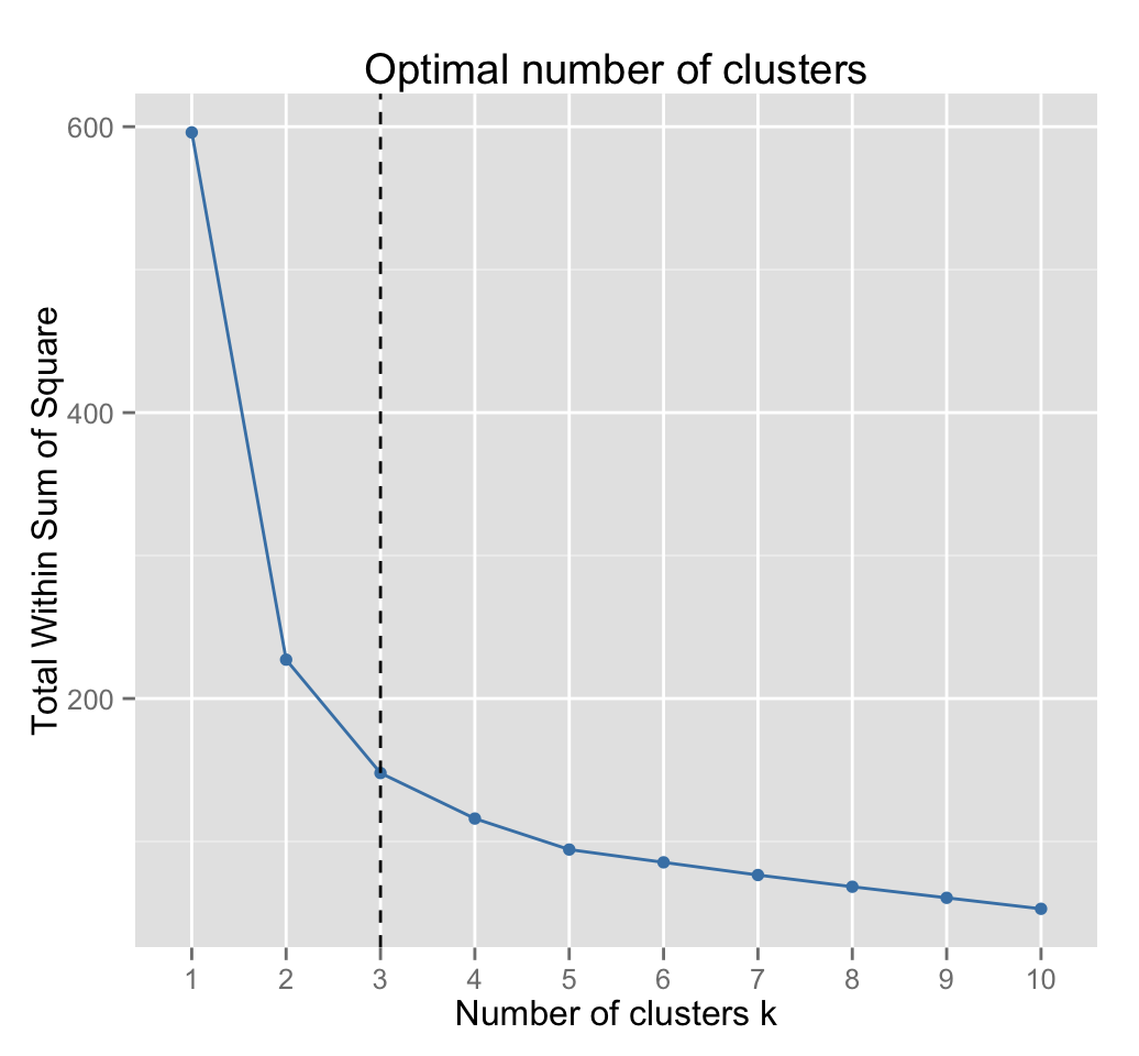
Three clusters are suggested.
Note that, the elbow method is sometimes ambiguous. An alternative is the average silhouette method (Kaufman and Rousseeuw [1990]) which can be also used with any clustering approach.
5.2 Average silhouette method
5.2.1 Concept
The average silhouette approach well be described comprehensively in the chapter cluster validation statistics. Briefly, it measures the quality of a clustering. That is, it determines how well each object lies within its cluster. A high average silhouette width indicates a good clustering.
Average silhouette method computes the average silhouette of observations for different values of k. The optimal number of clusters k is the one that maximize the average silhouette over a range of possible values for k (Kaufman and Rousseeuw [1990]).
5.2.2 Algorithm
The algorithm is similar to the elbow method and can be computed as follow:
- Compute clustering algorithm (e.g., k-means clustering) for different values of k. For instance, by varying k from 1 to 10 clusters
- For each k, calculate the average silhouette of observations (avg.sil)
- Plot the curve of avg.sil according to the number of clusters k.
- The location of the maximum is considered as the appropriate number of clusters.
5.2.3 R codes
The function silhouette() [in cluster package] is used to compute the average silhouette width.
5.2.3.1 Average silhouette method for k-means clustering
The R code below determine the optimal number of clusters K for k-means clustering:
library(cluster)
k.max <- 15
data <- iris.scaled
sil <- rep(0, k.max)

# Compute the average silhouette width for
# k = 2 to k = 15
for(i in 2:k.max){
  km.res <- kmeans(data, centers = i, nstart = 25)
  ss <- silhouette(km.res$cluster, dist(data))
  sil[i] <- mean(ss[, 3])
}

# Plot the  average silhouette width
plot(1:k.max, sil, type = "b", pch = 19,
     frame = FALSE, xlab = "Number of clusters k")
abline(v = which.max(sil), lty = 2)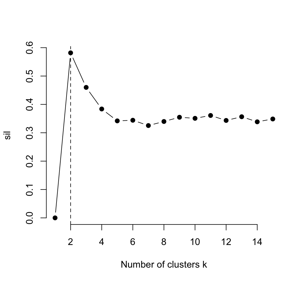
The function fviz_nbclust() [in factoextra package] can be also used. It just requires the cluster package to be installed:
require(cluster)
fviz_nbclust(iris.scaled, kmeans, method = "silhouette")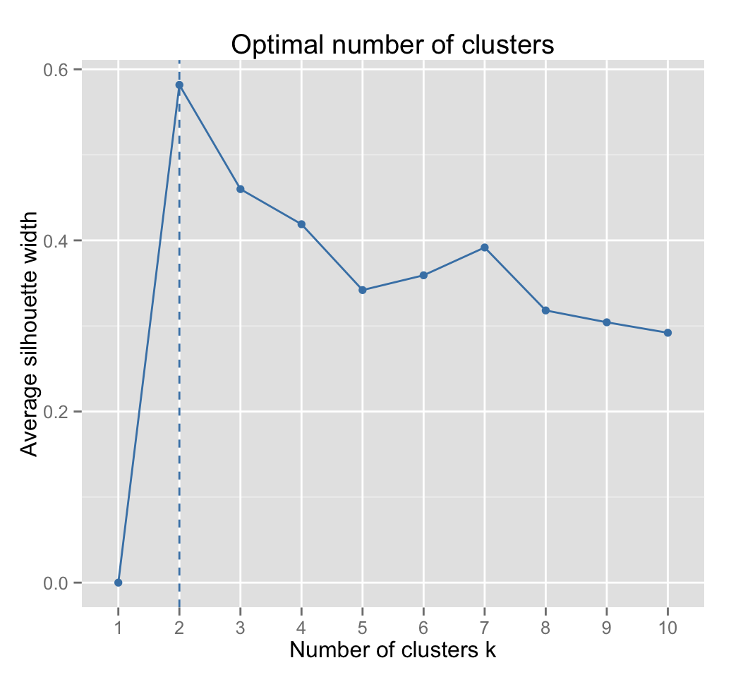
Two clusters are suggested.
5.2.3.2 Average silhouette method for PAM clustering
require(cluster)
fviz_nbclust(iris.scaled, pam, method = "silhouette")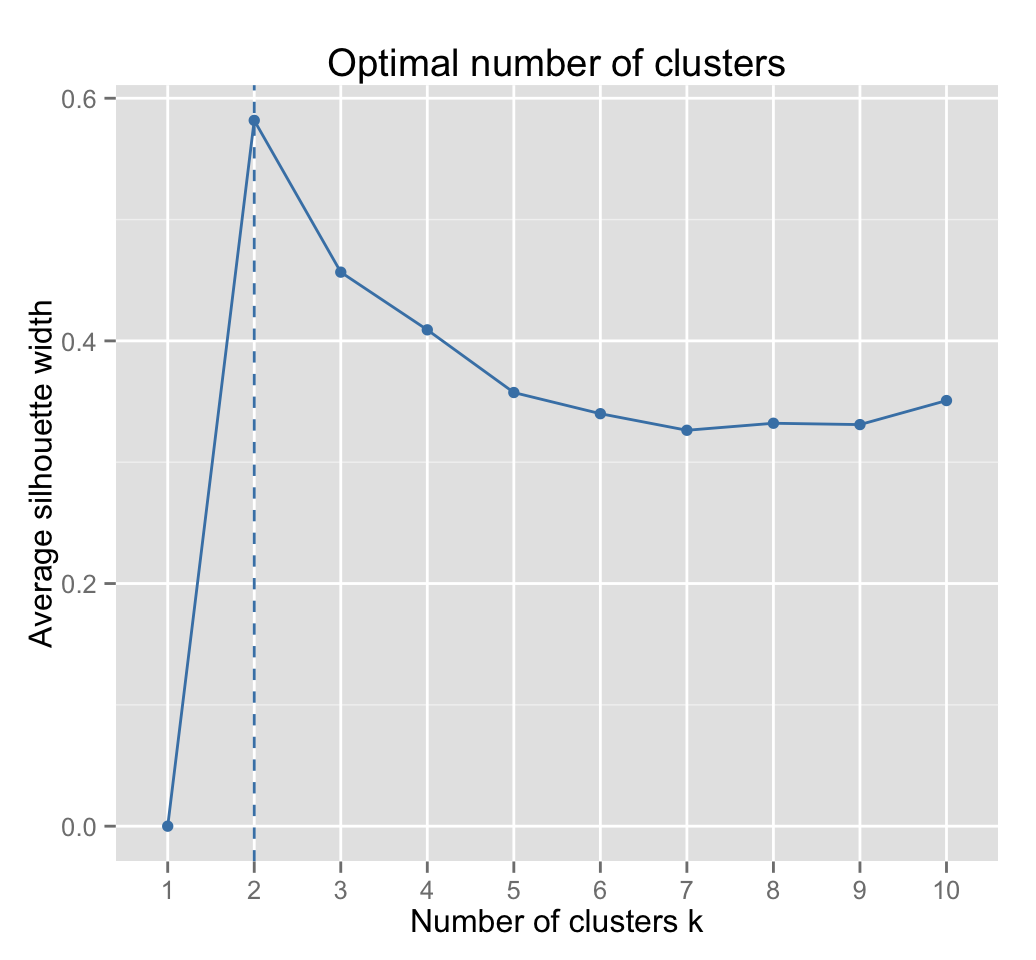
Two clusters are suggested.
5.2.3.3 Average silhouette method for hierarchical clustering
require(cluster)
fviz_nbclust(iris.scaled, hcut, method = "silhouette",
             hc_method = "complete")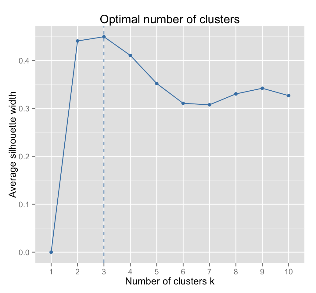
Three clusters are suggested.
5.3 Conclusions about elbow and silhouette methods
- Three cluster solutions are suggested using k-means, PAM and hierarchical clustering in combination with the elbow method.
- The average silhouette method gives two cluster solutions using k-means and PAM algorithms. Combining hierarchical clustering and silhouette method returns 3 clusters
According to these observations, its possible to define k = 3 as the optimal number of clusters in the data.
The disadvantage of elbow and average silhouette methods is that, they measure a global clustering characteristic only. A more sophisticated method is to use the gap statistic which provides a statistical procedure to formalize the elbow/silhouette heuristic in order to estimate the optimal number of clusters.
5.4 Gap statistic method
5.4.1 Concept
The gap statistic has been published by R. Tibshirani, G. Walther, and T. Hastie (Standford University, 2001). The approach can be applied to any clustering method (K-means clustering, hierarchical clustering, ).
The gap statistic compares the total within intracluster variation for different values of k with their expected values under null reference distribution of the data, i.e. a distribution with no obvious clustering.
Recall that, the total within intra-cluster variation for a given k clusters is the total within sum of square (\(w_k\)).
The reference dataset is generated using Monte Carlo simulations of the sampling process. That is, for each variable (\(x_i\)) in the data set we compute its range [\(min(x_i), max(x_j)\)] and generate values for the n points uniformly from the interval min to max.
Note that, the function runif(n, min, max) can be used to generate random uniform distribution.
For the observed data and the the reference data, the total intracluster variation is computed using different values of k. The gap statistic for a given k is defined as follow:
\[ Gap_n(k) = E_n^*\{log(W_k)\} - log(W_k) \]
Where \(E_n^*\) denotes the expectation under a sample of size \(n\) from the reference distribution. \(E_n^*\) is defined via bootstrapping (B) by generating B copies of the reference datasets and, by computing the average \(log(W_k^*)\).
Note that, the logarithm of the \(W_k\) values is used, as they can be quite large.
The gap statistic measures the deviation of the observed \(W_k\) value from its expected value under the null hypothesis.
The estimate of the optimal clusters \(\hat{k}\) will be value that maximize \(Gap_n(k)\) (i.e, that yields the largest gap statistic). This means that the clustering structure is far away from the uniform distribution of points.
Note that, using B = 500 gives quite precise results so that the gap plot is basically unchanged after an another run.
The standard deviation (\(sd_k\)) of \(log(W_k^*)\) is also computed in order to define the standard error (\(s_k\)) of the simulation as follow:
\[ s_k = sd_k \times \sqrt{1 + 1/B} \]
Finally, a more robust approach is to choose the optimal number of clusters K as the smallest k such that:
\[Gap(k) \geq Gap(k+1) - s_{k+1}\]
That is, we choose the smallest value of k such that the gap statistic is within one standard deviation of the gap at k+1.5.4.2 Algorithm
The algorithm involves the following steps (Read the original paper of the gap statistic):
- Cluster the observed data, varying the number of clusters from k = 1, , \(k_{max}\), and compute the corresponding \(W_k\).
- Generate B reference data sets and cluster each of them with varying number of clusters k = 1, , \(k_{max}\). Compute the estimated gap statistic \(Gap(k) = \frac{1}{B} \sum\limits_{b=1}^B log(W_{kb}^*) - log(W_k)\).
- Let \(\bar{w} = (1/B) \sum_b log(W^*_{kb})\), compute the standard deviation \(sd(k) = \sqrt{(1/B) \sum_b (log(W^*_{kb}) - \bar{w})^2}\) and define \(s_k = sd_k \times \sqrt{1 + 1/B}\).
- Choose the number of clusters as the smallest k such that \(Gap(k) \geq Gap(k+1) - s_{k+1}\).
5.4.3 R codes
5.4.3.1 R function for computing the gap statistic
The R function clusGap() [in cluster package ] can be used to estimate the number of clusters in the data by applying the gap statistic.
A simplified format is:
clusGap(x, FUNcluster, K.max, B = 100, verbose = TRUE, ...)- x: numeric matrix or data frame
- FUNcluster: a function (e.g.: kmeans, pam, ) which accepts i) a data matrix like x as first argument; ii) the number of clusters desired (k > = 2) as a second argument; and returns a list containing a component named cluster which is a vector of length \(n = nrow(x)\) of integers in 1:k determining the clustering or grouping of the n observations.
- K.max: the maximum number of clusters to consider, must be at least two.
- B: the number of Monte Carlo (bootstrap) samples.
- verbose: if TRUE, the computing progression is shown.
- : Further arguments for FUNcluster(), see kmeans example below.
clusGap() function returns an object of class clusGap which main component is Tab with K.max rows and 4 columns, named logW, E.logW, gap and SE.sim. Recall that \(gap = E.logW - logW\) and SE.sim is the standard error of gap.
5.4.3.2 Gap statistic for k-means clustering
The R code below shows some example using the clustGap() function.
Well use B = 50 to keep the function speedy. Note that, its recommended to use B = 500 for your analysis.
The output of clusGap() function can be visualized using the function fviz_gap_stat() [in factoextra].
# Compute gap statistic
library(cluster)
set.seed(123)
gap_stat <- clusGap(iris.scaled, FUN = kmeans, nstart = 25,
                    K.max = 10, B = 50)

# Print the result
print(gap_stat, method = "firstmax")
## Clustering Gap statistic ["clusGap"].
## B=50 simulated reference sets, k = 1..10
## --> Number of clusters (method 'firstmax'): 3
## logW E.logW gap SE.sim
## [1,] 4.534565 4.754595 0.2200304 0.02504585
## [2,] 4.021316 4.489687 0.4683711 0.02742112
## [3,] 3.806577 4.295715 0.4891381 0.02384746
## [4,] 3.699263 4.143675 0.4444115 0.02093871
## [5,] 3.589284 4.052262 0.4629781 0.02036366
## [6,] 3.519726 3.972254 0.4525278 0.02049566
## [7,] 3.448288 3.905945 0.4576568 0.02106987
## [8,] 3.398210 3.850807 0.4525967 0.01969193
## [9,] 3.334279 3.802315 0.4680368 0.01905974
## [10,] 3.250246 3.759661 0.5094149 0.01928183# Base plot of gap statistic
plot(gap_stat, frame = FALSE, xlab = "Number of clusters k")
abline(v = 3, lty = 2)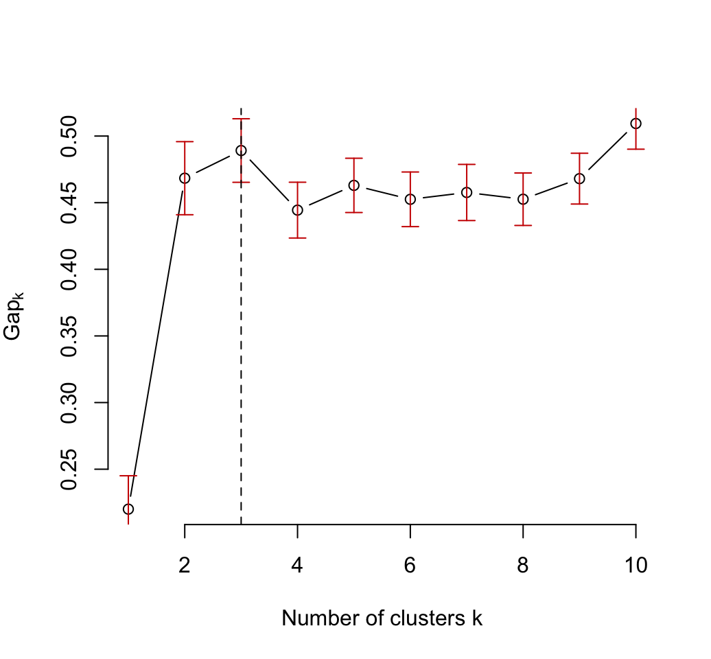
# Use factoextra
fviz_gap_stat(gap_stat)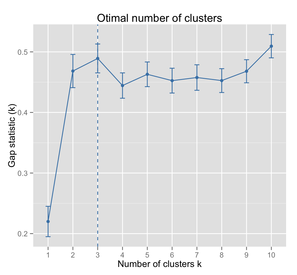
In our example, the algorithm suggests k = 3
The optimal number of clusters, k, is computed using the firstmax method (see ?cluster::maxSE). The criterion proposed by Tibshirani et al (2001) can be used as follow:
# Print
print(gap_stat, method = "Tibs2001SEmax")
# Plot
fviz_gap_stat(gap_stat,
              maxSE = list(method = "Tibs2001SEmax"))
# Relaxed the gap test to be within two standard deviations
fviz_gap_stat(gap_stat,
          maxSE = list(method = "Tibs2001SEmax", SE.factor = 2))
5.4.3.3 Gap statistic for PAM clustering
We dont need the argument nstart which is specific to kmeans() function.
# Compute gap statistic
set.seed(123)
gap_stat <- clusGap(iris.scaled, FUN = pam, K.max = 10, B = 50)
# Plot gap statistic
fviz_gap_stat(gap_stat)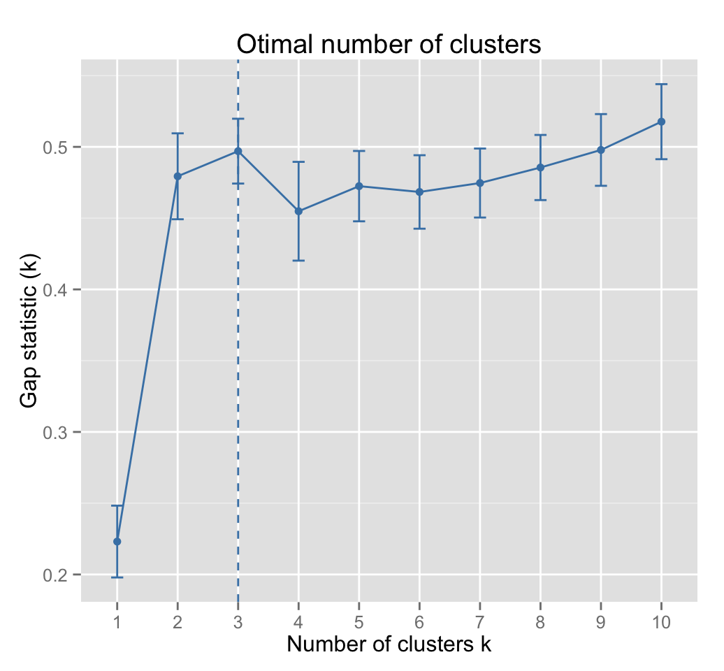
Three cluster solutions are suggested.
5.4.3.4 Gap statistic for hierarchical clustering
# Compute gap statistic
set.seed(123)
gap_stat <- clusGap(iris.scaled, FUN = hcut, K.max = 10, B = 50)
# Plot gap statistic
fviz_gap_stat(gap_stat)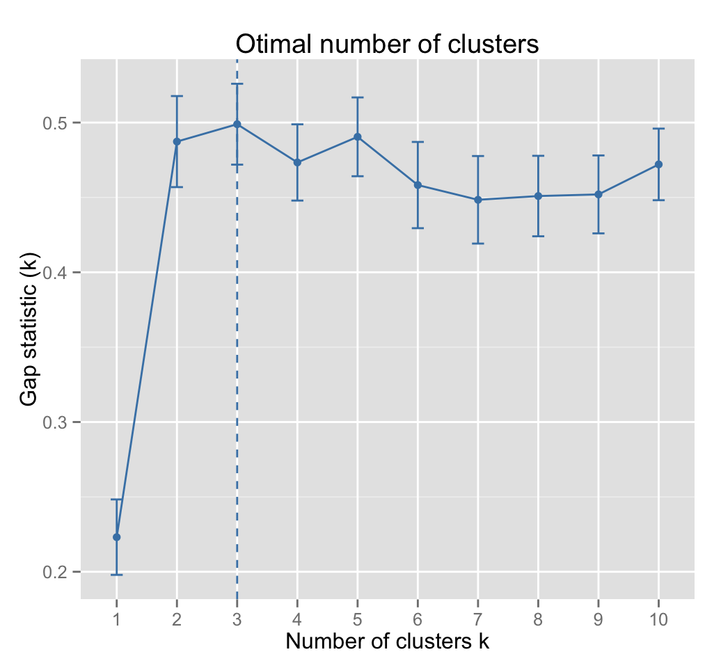
Three cluster solutions are suggested.
6 NbClust: A Package providing 30 indices for determining the best number of clusters
6.1 Overview of NbClust package
As mentioned in the introduction of this article, many indices have been proposed in the literature for determining the optimal number of clusters in a partitioning of a data set during the clustering process.
NbClust package, published by Charrad et al., 2014, provides 30 indices for determining the relevant number of clusters and proposes to users the best clustering scheme from the different results obtained by varying all combinations of number of clusters, distance measures, and clustering methods.
An important advantage of NbClust is that the user can simultaneously computes multiple indices and determine the number of clusters in a single function call.
The indices provided in NbClust package includes the gap statistic, the silhouette method and 28 other indices described comprehensively in the original paper of Charrad et al., 2014.
6.2 NbClust R function
The simplified format of the function NbClust() is:
NbClust(data = NULL, diss = NULL, distance = "euclidean",
min.nc = 2, max.nc = 15, method = NULL, index = "all")- data: matrix
- diss: dissimilarity matrix to be used. By default, diss=NULL, but if it is replaced by a dissimilarity matrix, distance should be NULL
- distance: the distance measure to be used to compute the dissimilarity matrix. Possible values include euclidean, manhattan or NULL.
- min.nc, max.nc: minimal and maximal number of clusters, respectively
- method: The cluster analysis method to be used including ward.D, ward.D2, single, complete, average and more
- index: the index to be calculated including silhouette, gap and more.
The value of NbClust() function includes the following elements:
- All.index: Values of indices for each partition of the dataset obtained with a number of clusters between min.nc and max.nc
- All.CriticalValues: Critical values of some indices for each partition obtained with a number of clusters between min.nc and max.nc
- Best.nc: Best number of clusters proposed by each index and the corresponding index value
- Best.partition: Partition that corresponds to the best number of clusters
6.3 Examples of usage
Note that, user can request indices one by one, by setting the argument index to the name of the index of interest, for example index = gap.
In this case, NbClust function displays:
- the gap statistic values of the partitions obtained with number of clusters varying from min.nc to max.nc ($All.index)
- the optimal number of clusters ($Best.nc)
- and the partition corresponding to the best number of clusters ($Best.partition)
6.3.1 Compute only an index of interest
The following example determine the number of clusters using gap statistics:
library("NbClust")
set.seed(123)
res.nb <- NbClust(iris.scaled, distance = "euclidean",
                  min.nc = 2, max.nc = 10,
                  method = "complete", index ="gap")
res.nb # print the results
## $All.index
## 2 3 4 5 6 7 8 9 10
## -0.2899 -0.2303 -0.6915 -0.8606 -1.0506 -1.3223 -1.3303 -1.4759 -1.5551
##
## $All.CriticalValues
## 2 3 4 5 6 7 8 9 10
## -0.0539 0.4694 0.1787 0.2009 0.2848 0.0230 0.1631 0.0988 0.1708
##
## $Best.nc
## Number_clusters Value_Index
## 3.0000 -0.2303
##
## $Best.partition
## [1] 1 1 1 1 1 1 1 1 1 1 1 1 1 1 1 1 1 1 1 1 1 1 1 1 1 1 1 1 1 1 1 1 1 1 1
## [36] 1 1 1 1 1 1 2 1 1 1 1 1 1 1 1 3 3 3 2 3 2 3 2 3 2 2 3 2 3 3 3 3 2 2 2
## [71] 3 3 3 3 3 3 3 3 3 2 2 2 2 3 3 3 3 2 3 2 2 3 2 2 2 3 3 3 2 2 3 3 3 3 3
## [106] 3 2 3 3 3 3 3 3 3 3 3 3 3 3 2 3 3 3 3 3 3 3 3 3 3 3 3 3 3 3 3 3 3 3 3
## [141] 3 3 3 3 3 3 3 3 3 3The elements returned by the function NbClust() are accessible using the R code below:
# All gap statistic values
res.nb$All.index

# Best number of clusters
res.nb$Best.nc

# Best partition
res.nb$Best.partition
6.3.2 Compute all the 30 indices
The following example compute all the 30 indices, in a single function call, for determining the number of clusters and suggests to user the best clustering scheme. The description of the indices are available in NbClust documentation (see ?NbClust).
To compute multiple indices simultaneously, the possible values for the argument index can be i) alllong or ii) all. The option alllong requires more time, as the run of some indices, such as Gamma, Tau, Gap and Gplus, is computationally very expensive. The user can avoid computing these four indices by setting the argument index to all. In this case, only 26 indices are calculated.
With the alllong option, the output of the NbClust function contains:
- all validation indices
- critical values for Duda, Gap, PseudoT2 and Beale indices
- the number of clusters corresponding to the optimal score for each indice
- the best number of clusters proposed by NbClust according to the majority rule
- the best partition
The R code below computes NbClust() with index = all:
nb <- NbClust(iris.scaled, distance = "euclidean", min.nc = 2,
        max.nc = 10, method = "complete", index ="all")
# Print the result
nbIts possible to visualize the result using the function fviz_nbclust() [in factoextra], as follow:
fviz_nbclust(nb) + theme_minimal()## Among all indices:
## ===================
## * 2 proposed 0 as the best number of clusters
## * 1 proposed 1 as the best number of clusters
## * 2 proposed 2 as the best number of clusters
## * 18 proposed 3 as the best number of clusters
## * 3 proposed 10 as the best number of clusters
##
## Conclusion
## =========================
## * Accoridng to the majority rule, the best number of clusters is 3 .
- .
- 2 proposed 2 as the best number of clusters
- 18 indices proposed 3 as the best number of clusters.
- 3 proposed 10 as the best number of clusters
7 Infos
This analysis has been performed using R software (ver. 3.2.1)
- Charrad M., Ghazzali N., Boiteau V., Niknafs A. (2014). NbClust: An R Package for Determining the Relevant Number of Clusters in a Data Set. Journal of Statistical Software, 61(6), 1-36.
- Kaufman, L. and Rousseeuw, P.J. (1990). Finding Groups in Data: An Introduction to Cluster Analysis. Wiley, New York.
- Tibshirani, R., Walther, G. and Hastie, T. (2001). Estimating the number of data clusters via the Gap statistic. Journal of the Royal Statistical Society B, 63, 411423. PDF