There are three standards methods for exploring multidimensional data:
- Principal component methods, used to summarize and to visualize the information contained in a multivariate data table. Individuals and variables with same profiles are grouped together in the plot. Principal component methods include:
- Principal Component Analysis (PCA), used for analyzing a data set containing continuous variables
- Correspondence Analysis (CA), an extension of PCA suited to handle a contingency table formed by two qualitative variables (or categorical data).
- Multiple Correspondence Analysis (MCA), an extension of simple CA for analyzing a data table containing more than two categorical variables.
- Hierarchical Clustering, used for identifying groups of similar observations in a data set.
- Partitioning clustering such as k-means, used for splitting a data set into several groups.
In my previous article, Hybrid hierarchical k-means clustering, I described HOW and WHY, we should combine hierarchical clustering and k-means clustering.
In the present article, I will show how to combine the three methods: principal component methods, hierarchical clustering and partitioning methods such as k-means to better describe and visualize the similarity between observations. The approach described here has been implemented in the R package FactoMineR (F. Husson et al., 2010). Its named HCPC for Hierarchical Clustering on Principal Components.
1 Why combining principal component and clustering methods?
1.1 Case of continuous variables: Use PCA as denoising step
In the case of a multidimensional data set containing continuous variables, principal component analysis (PCA) can be used to reduce the dimensionality of the data into few continuous variables (i.e, principal components) containing the most important information in the data.
PCA step can be considered as denoising step which can lead to a more stable clustering. This is very useful if you have a large data set with multiple variables, such as in gene expression data.
1.2 Case of categorical variables: Use CA or MCA before clustering
CA (for analyzing contingency table formed by two categorical variables) and MCA (for analyzing multidimensional categorical variables) can be used to transform categorical variables into a set of few continuous variables (the principal components) and to remove the noise in the data.
CA and MCA can be considered as pre-processing steps which allow to compute clustering on categorical data
2 Algorithm of hierachical clustering on principal component (HCPC)
- Compute principal component methods
- Use Principal Component Analysis (PCA) for continuous variables
- Use Correspondence Analysis (CA) for a contingency table formed by two categorical variables
- Use Multiple Correspondence Analysis (MCA) for a data set containing multiple categorical variables.
Compute hierarchical clustering: Hierarchical Clustering is performed using Wards criterion on the selected principal components. Ward criterion has to be used in the hierarchical clustering because it is based on the multidimensional variance (i.e.inertia) as well as principal component analysis.
Choose the number of clusters based on the hierarchical tree: An initial partitioning is performed by cutting the hierarchical tree.
- K-means clustering is performed to improve the initial partition obtained from hierarchical clustering. The final partitioning solution, obtained after consolidation with k-means, can be (slightly) different from the one obtained with the hierarchical clustering. The importance of combining hierarchical clustering and k-means clustering has been described in my previous post: Hybrid hierarchical k-means clustering
3 Computing HCPC in R
3.1 Required R packages
Well use FactoMineR for computing HCPC() and factoextra for data visualizations.
Install factoextra package as follow:
if(!require(devtools)) install.packages("devtools")
devtools::install_github("kassambara/factoextra")
FactoMineR can be installed as follow:
install.packages("FactoMineR")Load the packages:
library(factoextra)
library(FactoMineR)
3.2 R function for HCPC
The function HCPC()[in FactoMineR package] can be used to compute hierarchical clustering on principal components.
A simplified format is:
HCPC(res, nb.clust = 0, iter.max = 10, min = 3, max = NULL, graph = TRUE)- res: a PCA result or a data frame
- nb.clust: an integer specifying the number of clusters. Possible values are:
- 0: the tree is cut at the level the user clicks on
- -1: the tree is automatically cut at the suggested level
- Any positive integer: the tree is cut with nb.clusters clusters
- iter.max: the maximum number of iterations for k-means
- min, max: the minimum and the maximum number of clusters to be generated, respectively
- graph: if TRUE, graphics are displayed
3.3 Case of continuous variables
We start by computing again the principal component analysis(PCA) is performed on the data set. The argument ncp = 3 is used in the function PCA() to keep only the first three principal components. Next HCPC is applied on the result of the PCA.
3.3.1 Data preparation
Well use USArrest data set and we start by scaling the data:
# Load the data
data(USArrests)
# Scale the data
df <- scale(USArrests)
head(df)
## Murder Assault UrbanPop Rape
## Alabama 1.24256408 0.7828393 -0.5209066 -0.003416473
## Alaska 0.50786248 1.1068225 -1.2117642 2.484202941
## Arizona 0.07163341 1.4788032 0.9989801 1.042878388
## Arkansas 0.23234938 0.2308680 -1.0735927 -0.184916602
## California 0.27826823 1.2628144 1.7589234 2.067820292
## Colorado 0.02571456 0.3988593 0.8608085 1.864967207If you want to understand why the data are scaled before the analysis, then you should read this section: Distances and scaling.
3.3.2 Compute principal component analysis
Well use the package FactoMineR for computing HCPC and factoextra for the visualization of the output.
# Compute principal component analysis
library(FactoMineR)
res.pca <- PCA(USArrests, ncp = 5, graph=FALSE)
# Percentage of information retained by each
# dimensions
library(factoextra)
fviz_eig(res.pca)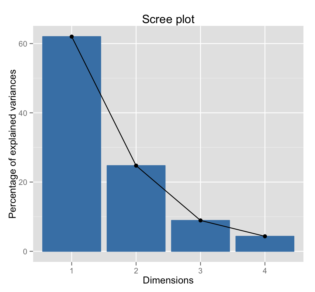
# Visualize variables
fviz_pca_var(res.pca)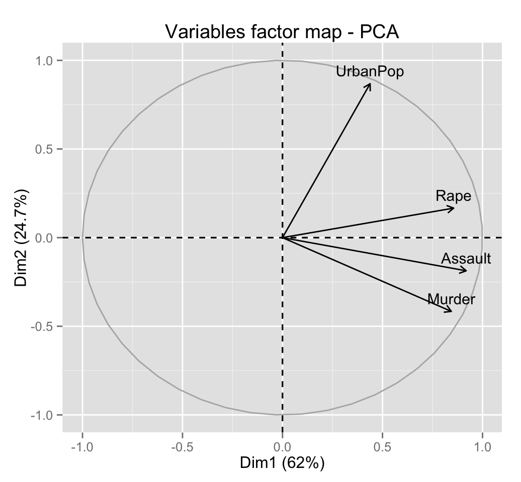
# Visualize individuals
fviz_pca_ind(res.pca)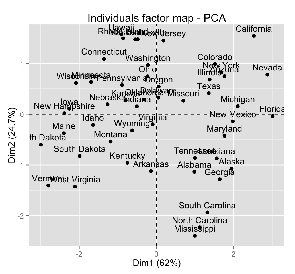
The first three dimensions of the PCA retains 96% of the total variance (i.e information) contained in the data:
get_eig(res.pca)## eigenvalue variance.percent cumulative.variance.percent
## Dim.1 2.4802416 62.006039 62.00604
## Dim.2 0.9897652 24.744129 86.75017
## Dim.3 0.3565632 8.914080 95.66425
## Dim.4 0.1734301 4.335752 100.00000Read more about PCA: Principal Component Analysis (PCA)
3.3.3 Compute hierarchical clustering on the PCA results
The function HCPC() is used:
# Compute PCA with ncp = 3
res.pca <- PCA(USArrests, ncp = 3, graph = FALSE)
# Compute HCPC
res.hcpc <- HCPC(res.pca, graph = FALSE)
The function HCPC() returns a list containing:
- data.clust: The original data with a supplementary row called class containing the partition.
- desc.var: The variables describing clusters
- call$t$res: The outputs of the principal component analysis
- call$t$tree: The outputs of agnes() function [in cluster package]
- call$t$nb.clust: The number of optimal clusters estimated
# Data with cluster assignements
head(res.hcpc$data.clust, 10)
## Murder Assault UrbanPop Rape clust
## Alabama 13.2 236 58 21.2 3
## Alaska 10.0 263 48 44.5 4
## Arizona 8.1 294 80 31.0 4
## Arkansas 8.8 190 50 19.5 3
## California 9.0 276 91 40.6 4
## Colorado 7.9 204 78 38.7 4
## Connecticut 3.3 110 77 11.1 2
## Delaware 5.9 238 72 15.8 2
## Florida 15.4 335 80 31.9 4
## Georgia 17.4 211 60 25.8 3# Variable describing clusters
res.hcpc$desc.var## $quanti.var
## Eta2 P-value
## Assault 0.7841402 2.376392e-15
## Murder 0.7771455 4.927378e-15
## Rape 0.7029807 3.480110e-12
## UrbanPop 0.5846485 7.138448e-09
##
## $quanti
## $quanti$`1`
## v.test Mean in category Overall mean sd in category Overall sd
## UrbanPop -3.898420 52.07692 65.540 9.691087 14.329285
## Murder -4.030171 3.60000 7.788 2.269870 4.311735
## Rape -4.052061 12.17692 21.232 3.130779 9.272248
## Assault -4.638172 78.53846 170.760 24.700095 82.500075
## p.value
## UrbanPop 9.682222e-05
## Murder 5.573624e-05
## Rape 5.076842e-05
## Assault 3.515038e-06
##
## $quanti$`2`
## v.test Mean in category Overall mean sd in category Overall sd
## UrbanPop 2.793185 73.87500 65.540 8.652131 14.329285
## Murder -2.374121 5.65625 7.788 1.594902 4.311735
## p.value
## UrbanPop 0.005219187
## Murder 0.017590794
##
## $quanti$`3`
## v.test Mean in category Overall mean sd in category Overall sd
## Murder 4.357187 13.9375 7.788 2.433587 4.311735
## Assault 2.698255 243.6250 170.760 46.540137 82.500075
## UrbanPop -2.513667 53.7500 65.540 7.529110 14.329285
## p.value
## Murder 1.317449e-05
## Assault 6.970399e-03
## UrbanPop 1.194833e-02
##
## $quanti$`4`
## v.test Mean in category Overall mean sd in category Overall sd
## Rape 5.352124 33.19231 21.232 6.996643 9.272248
## Assault 4.356682 257.38462 170.760 41.850537 82.500075
## UrbanPop 3.028838 76.00000 65.540 10.347798 14.329285
## Murder 2.913295 10.81538 7.788 2.001863 4.311735
## p.value
## Rape 8.692769e-08
## Assault 1.320491e-05
## UrbanPop 2.454964e-03
## Murder 3.576369e-03
##
##
## attr(,"class")
## [1] "catdes" "list "3.3.4 Visualize the results of HCPC using base plot
The function plot.HCPC() [in FactoMineR] is used:
plot(x, axes = c(1,2), choice = "3D.map",
     draw.tree = TRUE, ind.names = TRUE, title = NULL,
tree.barplot = TRUE, centers.plot = FALSE)- x: an object of class HCPC
- axes: the principal components to be plotted
- choice: a string. Possible values are:
- tree: plots the tree (dendrogram)
- bar: plots bars of inertia gains
- map: plots a factor map. Individuals are colored by cluster
- 3D.map: plots the factor map. The tree is added on the plot
- draw.tree: a logical value. If TRUE, the tree is plotted on the factor map if choice = map
- ind.names: a logical value. If TRUE, individual names are shown
- title: the title of the grap
- tree.barplot: a logical value. If TRUE, the barplot of intra inertia losses is added on the tree graph.
- centers.plot: a logical value. If TRUE, the centers of clusters are drawn on the factor maps
# Principal components + tree
plot(res.hcpc, choice = "3D.map")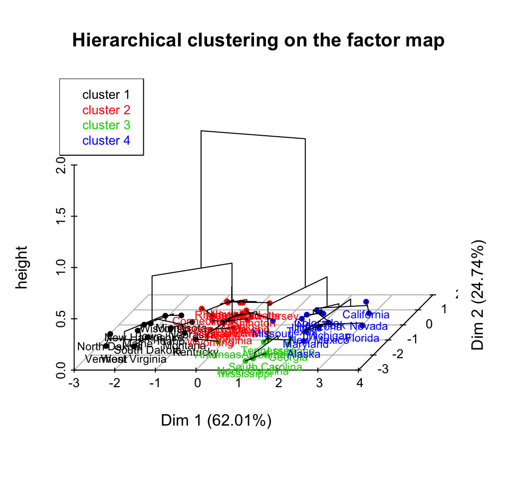
# Plot the dendrogram only
plot(res.hcpc, choice ="tree", cex = 0.6)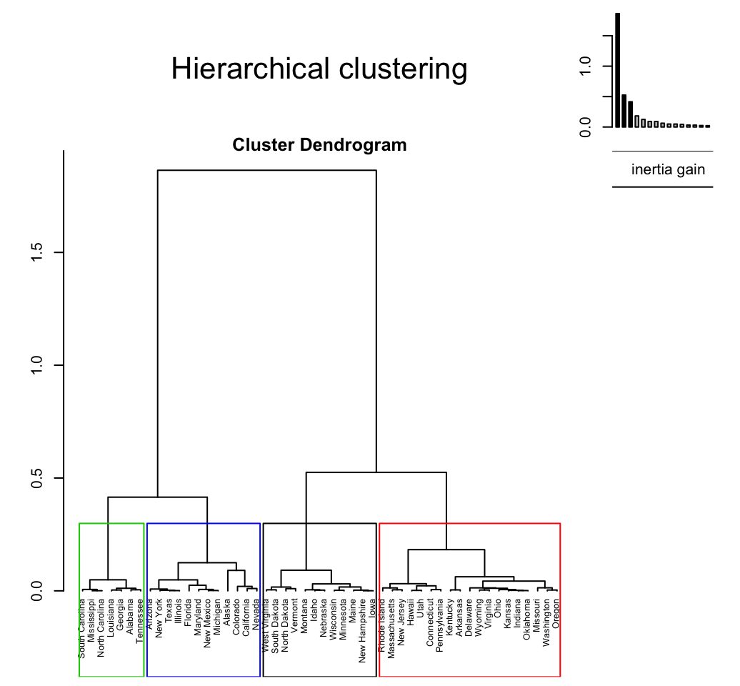
# Draw only the factor map
plot(res.hcpc, choice ="map", draw.tree = FALSE)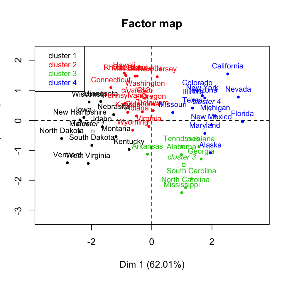
# Remove labels and add cluster centers
plot(res.hcpc, choice ="map", draw.tree = FALSE,
     ind.names = FALSE, centers.plot = TRUE)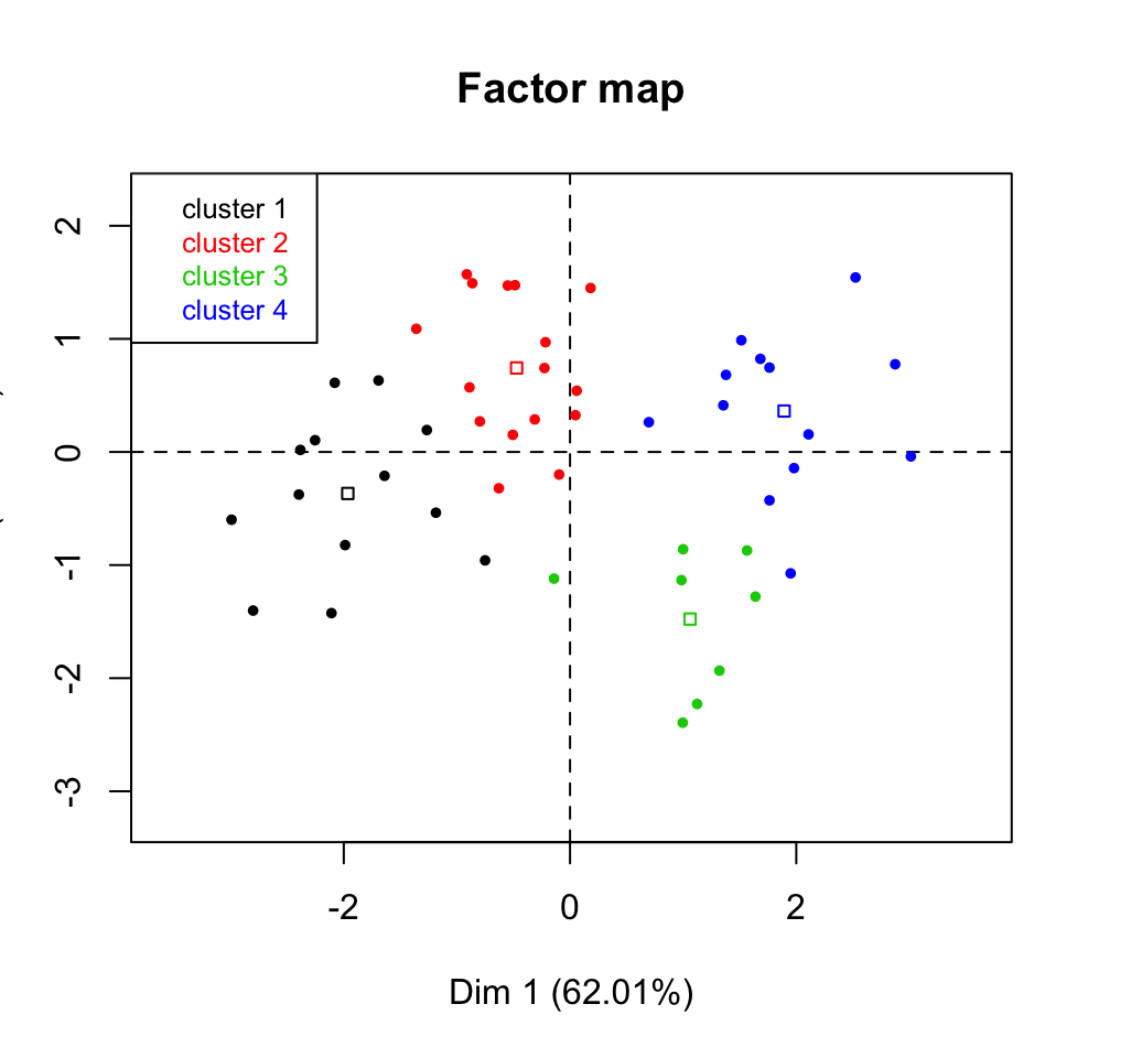
3.3.5 Visualize the results of HCPC using factoextra
The function fviz_cluster() can be used:
fviz_cluster(res.hcpc)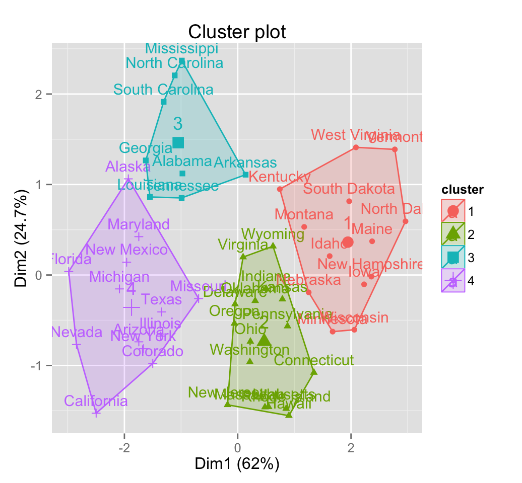
3.4 Case of categorical variables
Compute CA or MCA and then apply the function HCPC() on the results as described above. If you want to learn more about CA and MCA, read the following articles:
4 Infos
This analysis has been performed using R software (ver. 3.2.1)
- Husson, F., Josse, J. & Pagès J. (2010). Principal component methods - hierarchical clustering - partitional clustering: why would we need to choose for visualizing data?. Technical report. pdf