- 1 How this article is organized
- 2 Required R packages
- 3 Data preparation
- 4 R function for clustering analyses
- 5 Combining hierarchical clustering and k-means
- 5.1 Why?
- 5.2 How ?
- 5.3 R codes
- 5.3.1 Compute hierarchical clustering and cut the tree into k-clusters:
- 5.3.2 Compute the centers of clusters defined by hierarchical clustering:
- 5.3.3 K-means clustering using hierarchical clustering defined cluster-centers
- 5.3.4 Compare the results of hierarchical clustering and hybrid approach
- 5.3.5 Compare the results of standard k-means clustering and hybrid approach
- 5.4 hkmeans(): Easy-to-use function for hybrid hierarchical k-means clustering
- 6 Infos
Clustering algorithms are used to split a dataset into several groups (i.e clusters), so that the objects in the same group are as similar as possible and the objects in different groups are as dissimilar as possible.
The most popular clustering algorithms are:
- k-means clustering, a partitioning method used for splitting a dataset into a set of k clusters.
- hierarchical clustering, an alternative approach to k-means clustering for identifying clustering in the dataset by using pairwise distance matrix between observations as clustering criteria.
However, each of these two standard clustering methods has its limitations. K-means clustering requires the user to specify the number of clusters in advance and selects initial centroids randomly. Agglomerative hierarchical clustering is good at identifying small clusters but not large ones.
In this article, we document hybrid approaches for easily mixing the best of k-means clustering and hierarchical clustering.
1 How this article is organized
Well start by demonstrating why we should combine k-means and hierarcical clustering. An application is provided using R software.
Finally, well provide an easy to use R function (in factoextra package) for computing hybrid hierachical k-means clustering.
2 Required R packages
Well use the R package factoextra which is very helpful for simplifying clustering workflows and for visualizing clusters using ggplot2 plotting system
Install factoextra package as follow:
if(!require(devtools)) install.packages("devtools")
devtools::install_github("kassambara/factoextra")
Load the package:
library(factoextra)3 Data preparation
Well use USArrest dataset and we start by scaling the data:
# Load the data
data(USArrests)
# Scale the data
df <- scale(USArrests)
head(df)
## Murder Assault UrbanPop Rape
## Alabama 1.24256408 0.7828393 -0.5209066 -0.003416473
## Alaska 0.50786248 1.1068225 -1.2117642 2.484202941
## Arizona 0.07163341 1.4788032 0.9989801 1.042878388
## Arkansas 0.23234938 0.2308680 -1.0735927 -0.184916602
## California 0.27826823 1.2628144 1.7589234 2.067820292
## Colorado 0.02571456 0.3988593 0.8608085 1.864967207If you want to understand why the data are scaled before the analysis, then you should read this section: Distances and scaling.
4 R function for clustering analyses
Well use the function eclust() [in factoextra] which provides several advantages as described in the previous chapter: Visual Enhancement of Clustering Analysis.
eclust() stands for enhanced clustering. It simplifies the workflow of clustering analysis and, it can be used for computing hierarchical clustering and partititioning clustering in a single line function call.
4.1 Example of k-means clustering
Well split the data into 4 clusters using k-means clustering as follow:
library("factoextra")
# K-means clustering
km.res <- eclust(df, "kmeans", k = 4,
                 nstart = 25, graph = FALSE)
# k-means group number of each observation
head(km.res$cluster, 15)
## Alabama Alaska Arizona Arkansas California Colorado
## 4 3 3 4 3 3
## Connecticut Delaware Florida Georgia Hawaii Idaho
## 2 2 3 4 2 1
## Illinois Indiana Iowa
## 3 2 1# Visualize k-means clusters
fviz_cluster(km.res, frame.type = "norm", frame.level = 0.68)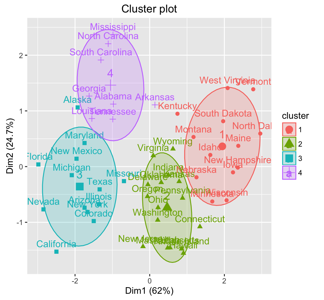
# Visualize the silhouette of clusters
fviz_silhouette(km.res)
## cluster size ave.sil.width
## 1 1 13 0.37
## 2 2 16 0.34
## 3 3 13 0.27
## 4 4 8 0.39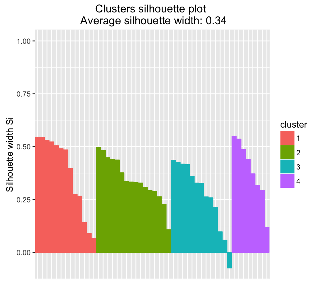
Note that, silhouette coefficient measures how well an observation is clustered and it estimates the average distance between clusters (i.e, the average silhouette width). Observations with negative silhouette are probably placed in the wrong cluster. Read more here: cluster validation statistics
Samples with negative silhouette coefficient:
# Silhouette width of observation
sil <- km.res$silinfo$widths[, 1:3]
# Objects with negative silhouette
neg_sil_index <- which(sil[, 'sil_width'] < 0)
sil[neg_sil_index, , drop = FALSE]
## cluster neighbor sil_width
## Missouri 3 2 -0.07318144Read more about k-means clustering: K-means clustering
4.2 Example of hierarchical clustering
# Enhanced hierarchical clustering
res.hc <- eclust(df, "hclust", k = 4,
                method = "ward.D2", graph = FALSE)
head(res.hc$cluster, 15)
## Alabama Alaska Arizona Arkansas California Colorado
## 1 2 2 3 2 2
## Connecticut Delaware Florida Georgia Hawaii Idaho
## 4 3 2 1 3 4
## Illinois Indiana Iowa
## 2 3 4# Dendrogram
fviz_dend(res.hc, rect = TRUE, show_labels = TRUE, cex = 0.5) 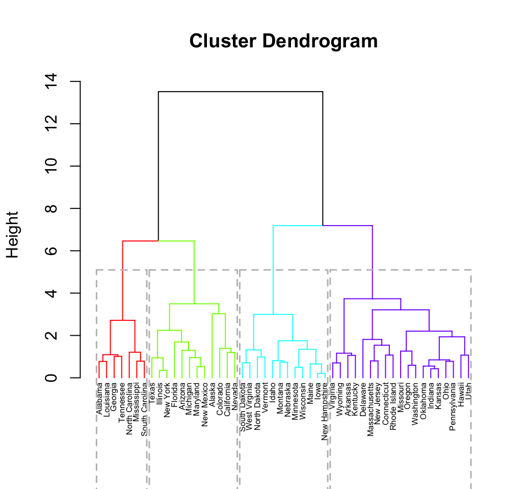
# Visualize the silhouette of clusters
fviz_silhouette(res.hc)
## cluster size ave.sil.width
## 1 1 7 0.40
## 2 2 12 0.26
## 3 3 18 0.38
## 4 4 13 0.35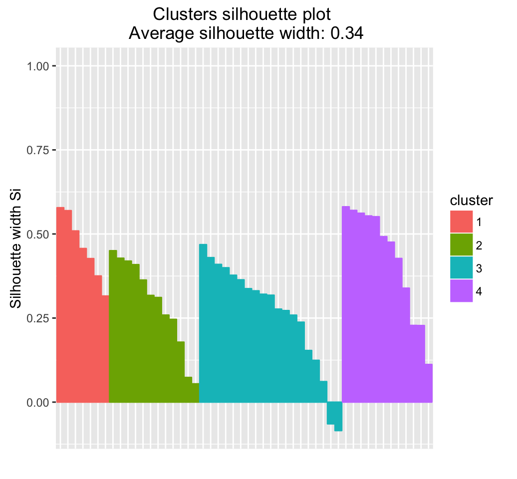
It can be seen that three samples have negative silhouette coefficient indicating that they are not in the right cluster. These samples are:
# Silhouette width of observation
sil <- res.hc$silinfo$widths[, 1:3]
# Objects with negative silhouette
neg_sil_index <- which(sil[, 'sil_width'] < 0)
sil[neg_sil_index, , drop = FALSE]
## cluster neighbor sil_width
## Alaska 2 1 -0.005212336
## Nebraska 4 3 -0.044172624
## Connecticut 4 3 -0.078016589Read more about hierarchical clustering: Hierarchical clustering
5 Combining hierarchical clustering and k-means
5.1 Why?
Recall that, in k-means algorithm, a random set of observations are chosen as the initial centers.
The final k-means clustering solution is very sensitive to this initial random selection of cluster centers. The result might be (slightly) different each time you compute k-means.
To avoid this, a solution is to use an hybrid approach by combining the hierarchical clustering and the k-means methods. This process is named hybrid hierarchical k-means clustering (hkmeans).
5.2 How ?
The procedure is as follow:
- Compute hierarchical clustering and cut the tree into k-clusters
- compute the center (i.e the mean) of each cluster
- Compute k-means by using the set of cluster centers (defined in step 3) as the initial cluster centers
Note that, k-means algorithm will improve the initial partitioning generated at the step 2 of the algorithm. Hence, the initial partitioning can be slightly different from the final partitioning obtained in the step 4.
5.3 R codes
5.3.1 Compute hierarchical clustering and cut the tree into k-clusters:
res.hc <- eclust(df, "hclust", k = 4,
                method = "ward.D2", graph = FALSE)
grp <- res.hc$cluster
5.3.2 Compute the centers of clusters defined by hierarchical clustering:
Cluster centers are defined as the means of variables in clusters. The function aggregate() can be used to compute the mean per group in a data frame.
# Compute cluster centers
clus.centers <- aggregate(df, list(grp), mean)
clus.centers
## Group.1 Murder Assault UrbanPop Rape
## 1 1 1.5803956 0.9662584 -0.7775109 0.04844071
## 2 2 0.7298036 1.1188219 0.7571799 1.32135653
## 3 3 -0.3250544 -0.3231032 0.3733701 -0.17068130
## 4 4 -1.0745717 -1.1056780 -0.7972496 -1.00946922# Remove the first column
clus.centers <- clus.centers[, -1]
clus.centers## Murder Assault UrbanPop Rape
## 1 1.5803956 0.9662584 -0.7775109 0.04844071
## 2 0.7298036 1.1188219 0.7571799 1.32135653
## 3 -0.3250544 -0.3231032 0.3733701 -0.17068130
## 4 -1.0745717 -1.1056780 -0.7972496 -1.009469225.3.3 K-means clustering using hierarchical clustering defined cluster-centers
km.res2 <- eclust(df, "kmeans", k = clus.centers, graph = FALSE)
fviz_silhouette(km.res2)
## cluster size ave.sil.width
## 1 1 8 0.39
## 2 2 13 0.27
## 3 3 16 0.34
## 4 4 13 0.37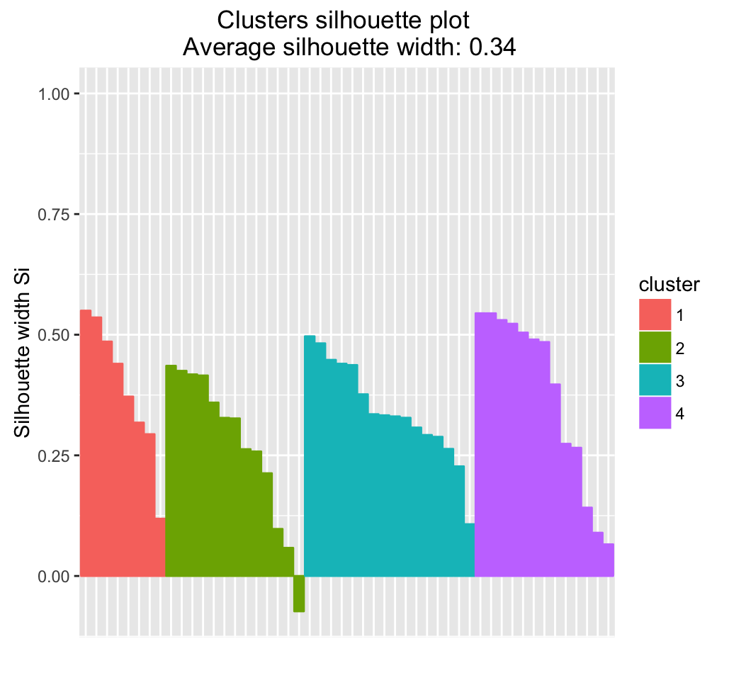
5.3.4 Compare the results of hierarchical clustering and hybrid approach
The R code below compares the initial clusters defined using only hierarchical clustering and the final ones defined using hierarchical clustering + k-means:
# res.hc$cluster: Initial clusters defined using hierarchical clustering
# km.res2$cluster: Final clusters defined using k-means
table(km.res2$cluster, res.hc$cluster)
##
## 1 2 3 4
## 1 7 0 1 0
## 2 0 12 1 0
## 3 0 0 15 1
## 4 0 0 1 12It can be seen that, 3 of the observations defined as belonging to cluster 3 by hierarchical clustering has been reclassified to cluster 1, 2, and 4 in the final solution defined by k-means clustering.
The difference can be easily visualized using the function fviz_dend() [in factoextra]. The labels are colored using k-means clusters:
fviz_dend(res.hc, k = 4,
          k_colors = c("blue", "green3", "red", "black"),
          label_cols =  km.res$cluster[res.hc$order], cex = 0.6)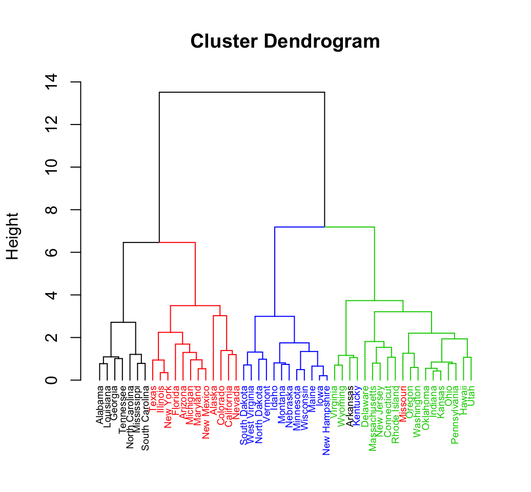
It can be seen that the hierarchical clustering result has been improved by the k-means algorithm.
5.3.5 Compare the results of standard k-means clustering and hybrid approach
# Final clusters defined using hierarchical k-means clustering
km.clust <- km.res$cluster

# Standard k-means clustering
set.seed(123)
res.km <- kmeans(df, centers = 4, iter.max = 100)


# comparison
table(km.clust, res.km$cluster)
##
## km.clust 1 2 3 4
## 1 13 0 0 0
## 2 0 16 0 0
## 3 0 0 13 0
## 4 0 0 0 8In our current example, there was no further improvement of the k-means clustering result by the hybrid approach. An improvement might be observed using another dataset.
5.4 hkmeans(): Easy-to-use function for hybrid hierarchical k-means clustering
The function hkmeans() [in factoextra] can be used to compute easily the hybrid approach of k-means on hierarchical clustering. The format of the result is similar to the one provided by the standard kmeans() function.
# Compute hierarchical k-means clustering
res.hk <-hkmeans(df, 4)
# Elements returned by hkmeans()
names(res.hk)
## [1] "cluster" "centers" "totss" "withinss"
## [5] "tot.withinss" "betweenss" "size" "iter"
## [9] "ifault" "data" "hclust"# Print the results
res.hk## Hierarchical K-means clustering with 4 clusters of sizes 8, 13, 16, 13
##
## Cluster means:
## Murder Assault UrbanPop Rape
## 1 1.4118898 0.8743346 -0.8145211 0.01927104
## 2 0.6950701 1.0394414 0.7226370 1.27693964
## 3 -0.4894375 -0.3826001 0.5758298 -0.26165379
## 4 -0.9615407 -1.1066010 -0.9301069 -0.96676331
##
## Clustering vector:
## Alabama Alaska Arizona Arkansas California
## 1 2 2 1 2
## Colorado Connecticut Delaware Florida Georgia
## 2 3 3 2 1
## Hawaii Idaho Illinois Indiana Iowa
## 3 4 2 3 4
## Kansas Kentucky Louisiana Maine Maryland
## 3 4 1 4 2
## Massachusetts Michigan Minnesota Mississippi Missouri
## 3 2 4 1 2
## Montana Nebraska Nevada New Hampshire New Jersey
## 4 4 2 4 3
## New Mexico New York North Carolina North Dakota Ohio
## 2 2 1 4 3
## Oklahoma Oregon Pennsylvania Rhode Island South Carolina
## 3 3 3 3 1
## South Dakota Tennessee Texas Utah Vermont
## 4 1 2 3 4
## Virginia Washington West Virginia Wisconsin Wyoming
## 3 3 4 4 3
##
## Within cluster sum of squares by cluster:
## [1] 8.316061 19.922437 16.212213 11.952463
## (between_SS / total_SS = 71.2 %)
##
## Available components:
##
##  [1] "cluster"      "centers"      "totss"        "withinss"
##  [5] "tot.withinss" "betweenss"    "size"         "iter"
##  [9] "ifault"       "data"         "hclust"
# Visualize the tree
fviz_dend(res.hk, cex = 0.6, rect = TRUE)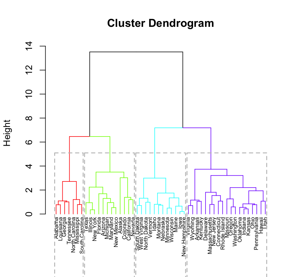
# Visualize the hkmeans final clusters
fviz_cluster(res.hk, frame.type = "norm", frame.level = 0.68)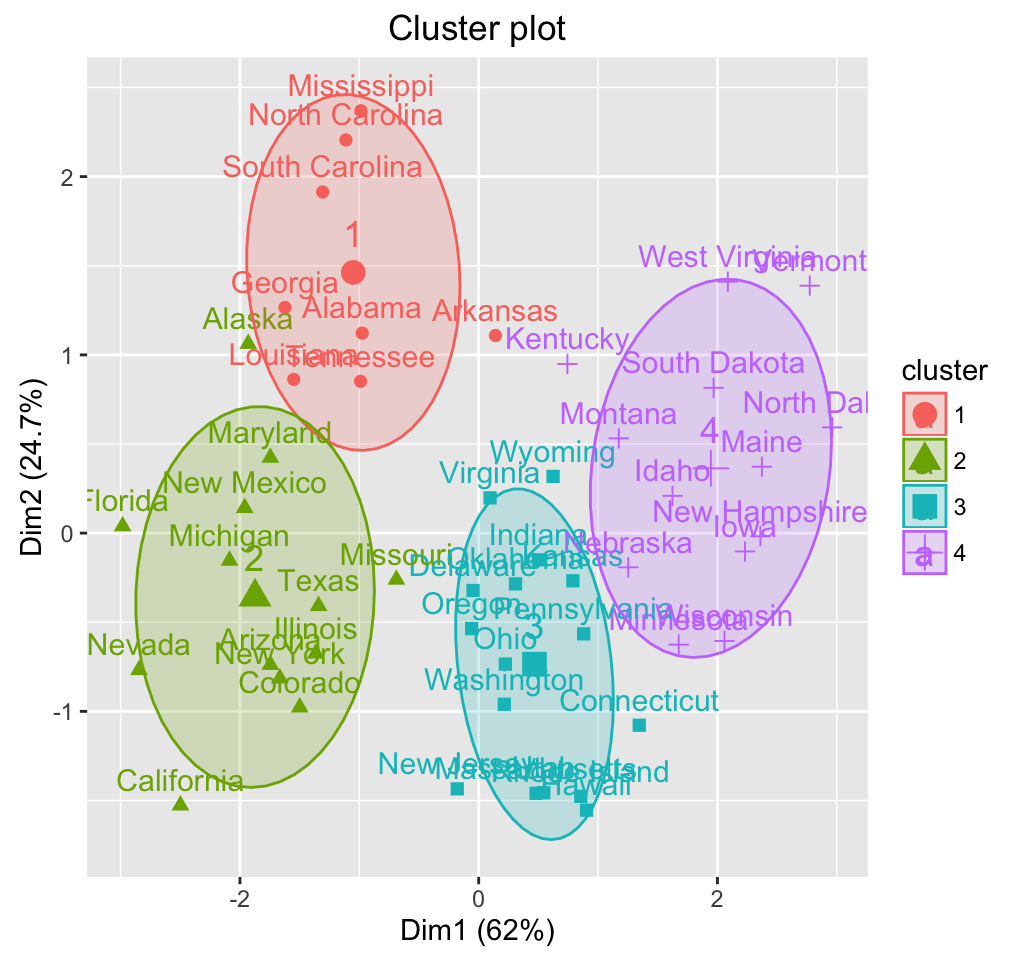
6 Infos
This analysis has been performed using R software (ver. 3.2.1)