Quantcast
Channel: Easy Guides
Viewing all 183 articles
Browse latest View live

Exporting Data From R

$
0
0


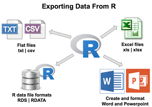
In the previous chapters we described the essentials of R programming as well as how to import data into R. Here, you’ll learn how to export data from R to txt, csv, Excel (xls, xlsx) and R data file formats. Additionally, we’ll describe how to create and format Word and PowerPoint documents from R.


Exporting data from R


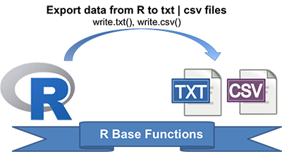
  1. Writing data from R to a txt|csv file: R base functions
  • R base functions for writing data: write.table(), write.csv(), write.csv2()
  • Writing data to a file


Writing Data From R to txt|csv Files: R Base Functions

# Loading mtcars data
data("mtcars")

# Write data to txt file: tab separated values
# sep = "\t"
write.table(mtcars, file = "mtcars.txt", sep = "\t",
            row.names = TRUE, col.names = NA)

# Write data to csv files:  
# decimal point = "." and value separators = comma (",")
write.csv(mtcars, file = "mtcars.csv")

# Write data to csv files: 
# decimal point = comma (",") and value separators = semicolon (";")
write.csv2(mtcars, file = "mtcars.csv")

Read more: Writing data from R to a txt|csv file: R base functions

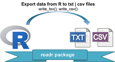
  1. Fast writing of Data From R to txt|csv Files: readr package
  • Installing and loading readr: install.packages(“readr”)
  • readr functions for writing data: write_tsv(), write_csv()
  • Writing data to a file


Fast Writing of Data From R to txt|csv Files: readr package

# Loading mtcars data
data("mtcars")

library("readr")
# Writing mtcars data to a tsv file
write_tsv(mtcars, path = "mtcars.txt")

# Writing mtcars data to a csv file
write_csv(mtcars, path = "mtcars.csv")

Read more: Fast writing of Data From R to txt|csv Files: readr package

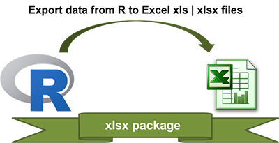
  1. Writing data from R to Excel files (xls|xlsx)
  • Installing xlsx package: install.packages(“xlsx”)
  • Using xlsx package: write.xlsx()


Writing Data From R to Excel Files (xls|xlsx)

library("xlsx")

# Write the first data set in a new workbook
write.xlsx(USArrests, file = "myworkbook.xlsx",
      sheetName = "USA-ARRESTS", append = FALSE)

# Add a second data set in a new worksheet
write.xlsx(mtcars, file = "myworkbook.xlsx", 
           sheetName="MTCARS", append=TRUE)

Read more: Writing data from R to Excel files (xls|xlsx)

  1. Saving data into R data format: RDATA and RDS
  • Save one object to a file: saveRDS(object, file), readRDS(file)
  • Save multiple objects to a file: save(data1, data2, file), load(file)
  • Save your entire workspace: save.image(), load()
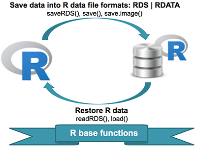

Save data into R data formats

  1. Saving and restoring one single R object:
# Save a single object to a file
saveRDS(mtcars, "mtcars.rds")

# Restore it under a different name
my_data <- readRDS("mtcars.rds")
  1. Saving and restoring one or more R objects:
# Save multiple objects
save(data1, data2, file = "data.RData")

# To load the data again
load("data.RData")
  1. Saving and restoring your entire workspace:
# Save your workspace
save.image(file = "my_work_space.RData")

# Load the workspace again
load("my_work_space.RData")

Read more: Saving data into R data format: RDATA and RDS

  1. Create and format Word documents with R and ReporteRs package

ReporteRs package, by David Gohel, provides easy to use functions to write and formatWord documents. It can be also used to generate Word document from a template file with logos, fonts, etc. ReporteRs is Java-based solution, so it works on Windows, Linux and Mac OS systems.

  • Install and load the ReporteRs R package
  • Create a simple Word document
    • Add texts : title and paragraphs of texts
    • Format the text of a Word document using R software
    • Add plots and images
    • Add a table
    • Add lists : ordered and unordered lists
    • Add a footnote to a Word document
    • Add R scripts
  • Add a table of contents into a Word document
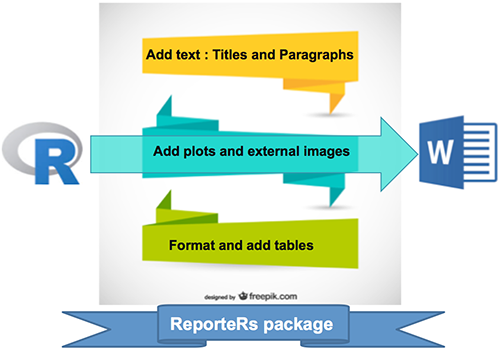

Write a Word document using R software and ReporteRs package

Read more: Create and format Word documents with R and ReporteRs package

  1. Create a Word document from a template file with R and ReporteRs package
  • Quick introduction to ReporteRs package
  • Create a Word document using a template file


Read and write a Word document from a template using R software and ReporteRs package

Read more: Create a Word document from a template file with R and ReporteRs package

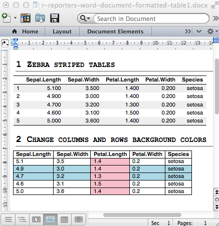
  1. Add a table into a Word document with R and ReporteRs package
  • Add a simple table
  • Add a formatted table
    • Change the background colors of rows and columns
    • Change cell background and text colors
    • Insert content into a table : header and footer rows
  • Analyze, format and export a correlation matrix into a Word document
  • Powerpoint


Add a table into a Word document with R and ReporteRs package

Read more: Add a table into a Word document with R and ReporteRs package

  1. Create and format PowerPoint documents with R and ReporteRs
  • Why is it important to be able to generate a PowerPoint report from R ?
    • Reason I : Many collaborators works with Microsoft office tools
    • Reason II : keeping beautiful R graphs beautiful for publications
  • Install and load the ReporteRs package
  • Create a simple PowerPoint document
    • Slide layout
    • Generate a simple PowerPoint document from R software
    • Format the text of a PowerPoint document
    • Add plots and images
    • Add a table
    • Add ordered and unordered lists
  • Create a PowerPoint document from a template file
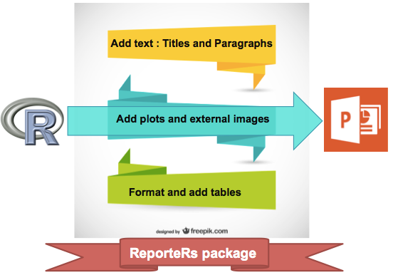

Write a PowerPoint document using R software and ReporteRs package

Write a PowerPoint document using R software and ReporteRs package

Read more: Create and format PowerPoint documents with R and ReporteRs

  1. Create an editable graph from R to PowerPoint
  • Case of base graphs
  • Case of graphs generated using ggplot2
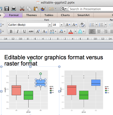

Editable plot from R software using ReporteRs package

Read more: Create an editable graph from R to PowerPoint


Importing Data Into R

$
0
0


In the previous chapter we described the essentials of R programming. Here, you’ll learn how to import data from txt, csv, Excel (xls, xlsx) into R.


Importing data into R


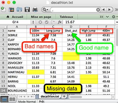
  1. Best practices in preparing data files for importing into R

Excel file

Read more: Best practices in preparing data files for importing into R

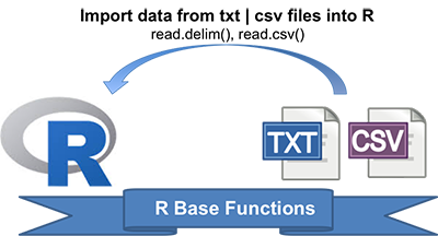
  1. Reading data from txt|csv files: R base functions
  • R base functions for importing data: read.table(), read.delim(), read.csv(), read.csv2()
  • Reading a local file
  • Reading a file from internet

Reading Data From txt|csv Files: R Base Functions

# Read tab separated values
read.delim(file.choose())

# Read comma (",") separated values
read.csv(file.choose())

# Read semicolon (";") separated values
read.csv2(file.choose())

Read more: Reading data from txt|csv files: R base functions


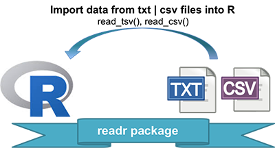
  1. Fast Reading of Data From txt|csv Files into R: readr package
  • Functions for reading txt|csv files: read_delim(), read_tsv(), read_csv(), read_csv2()
  • Reading a file
    • Reading a local file
    • Reading a file from internet
    • In the case of parsing problems
  • Specify column types
  • Reading lines from a file: read_lines()
  • Read whole file: read_file()

Reading Data From txt|csv Files: readr package

library("readr")

# Read tab separated values
read_tsv(file.choose())

# Read comma (",") separated values
read_csv(file.choose())

# Read semicolon (";") separated values
read_csv2(file.choose())

Read more: Fast Reading of Data From txt|csv Files into R: readr package


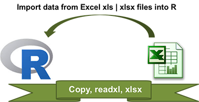
  1. Reading data From Excel Files (xls|xlsx) into R
  • Copying data from Excel and import into R
  • Importing Excel files into R using readxl package
  • Importing Excel files using xlsx package

Reading Data From Excel Files (xls|xlsx) into R

# Use readxl package to read xls|xlsx
library("readxl")
my_data <- read_excel("my_file.xlsx")

# Use xlsx package
library("xlsx")
my_data <- read.xlsx("my_file.xlsx") 

Read more: Reading data From Excel Files (xls|xlsx) into R


Preparing and Reshaping Data in R for Easier Analyses

$
0
0
About 80% of data analysis is spent on the process of cleaning and preparing the data (Dasu and Johnson 2003). Make sure that your data is in the right format for easier analysis in R.

Read the articles below

Data Manipulation in R

Tibble Data Format in R: Best and Modern Way to Work with Your Data

$
0
0


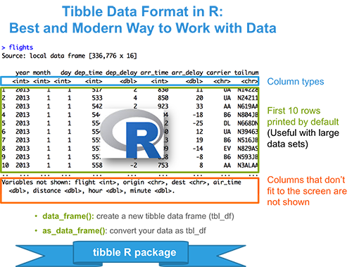
Previously, we described the essentials of R programming and provided quick start guides for importing data into R. The traditional R base functions read.table(), read.delim() and read.csv() import data into R as a data frame. However, the most modern R package readr provides several functions (read_delim(), read_tsv() and read_csv()), which are faster than R base functions and import data into R as a tbl_df (pronounced as “tibble diff”).

tbl_df object is a data frame providing a nicer printing method, useful when working with large data sets.


In this article, we’ll present the tibble R package, developed by Hadley Wickham. The tibble R package provides easy to use functions for creating tibbles, which is a modern rethinking of data frames.


tibble data format: tbl_df

Preleminary tasks

Launch RStudio as described here: Running RStudio and setting up your working directory

Installing and loading tibble package

# Installing
install.packages("tibble")

# Loading
library("tibble")

Create a new tibble

To create a new tibble from combining multiple vectors, use the function data_frame():

# Create
friends_data <- data_frame(
  name = c("Nicolas", "Thierry", "Bernard", "Jerome"),
  age = c(27, 25, 29, 26),
  height = c(180, 170, 185, 169),
  married = c(TRUE, FALSE, TRUE, TRUE)
)

# Print
friends_data
Source: local data frame [4 x 4]

     name   age height married
    <chr> <dbl>  <dbl>   <lgl>
1 Nicolas    27    180    TRUE
2 Thierry    25    170   FALSE
3 Bernard    29    185    TRUE
4  Jerome    26    169    TRUE

Compared to the traditional data.frame(), the modern data_frame():

  • never converts string as factor
  • never changes the names of variables
  • never create row names


Convert your data as a tibble

Note that, if you use the readr package to import your data into R, then you don’t need to do this step. readr imports already data as tbl_df.

To convert a traditional data as a tibble use the function as_data_frame() [in tibble package], which works on data frames, lists, matrices and tables:

library("tibble")

# Loading data
data("iris")
# Class of iris
class(iris)
[1] "data.frame"
# Print the frist 6 rows
head(iris, 6)
  Sepal.Length Sepal.Width Petal.Length Petal.Width Species
1          5.1         3.5          1.4         0.2  setosa
2          4.9         3.0          1.4         0.2  setosa
3          4.7         3.2          1.3         0.2  setosa
4          4.6         3.1          1.5         0.2  setosa
5          5.0         3.6          1.4         0.2  setosa
6          5.4         3.9          1.7         0.4  setosa
# Convert iris data to a tibble
my_data <- as_data_frame(iris)
class(my_data)
[1] "tbl_df"     "tbl"        "data.frame"
# Print my data
my_data
Source: local data frame [150 x 5]

   Sepal.Length Sepal.Width Petal.Length Petal.Width Species
          <dbl>       <dbl>        <dbl>       <dbl>  <fctr>
1           5.1         3.5          1.4         0.2  setosa
2           4.9         3.0          1.4         0.2  setosa
3           4.7         3.2          1.3         0.2  setosa
4           4.6         3.1          1.5         0.2  setosa
5           5.0         3.6          1.4         0.2  setosa
6           5.4         3.9          1.7         0.4  setosa
7           4.6         3.4          1.4         0.3  setosa
8           5.0         3.4          1.5         0.2  setosa
9           4.4         2.9          1.4         0.2  setosa
10          4.9         3.1          1.5         0.1  setosa
..          ...         ...          ...         ...     ...

Note that, only the first 10 rows are displayed

In the situation where you want to turn a tibble back to a data frame, use the function as.data.frame(my_data).

Advantages of tibbles compared to data frames

  1. Tibbles have nice printing method that show only the first 10 rows and all the columns that fit on the screen. This is useful when you work with large data sets.

  2. When printed, the data type of each column is specified (see below):
    • : for double
    • : for factor
    • : for character
    • : for logical
my_data
Source: local data frame [150 x 5]

   Sepal.Length Sepal.Width Petal.Length Petal.Width Species
          <dbl>       <dbl>        <dbl>       <dbl>  <fctr>
1           5.1         3.5          1.4         0.2  setosa
2           4.9         3.0          1.4         0.2  setosa
3           4.7         3.2          1.3         0.2  setosa
4           4.6         3.1          1.5         0.2  setosa
5           5.0         3.6          1.4         0.2  setosa
6           5.4         3.9          1.7         0.4  setosa
7           4.6         3.4          1.4         0.3  setosa
8           5.0         3.4          1.5         0.2  setosa
9           4.4         2.9          1.4         0.2  setosa
10          4.9         3.1          1.5         0.1  setosa
..          ...         ...          ...         ...     ...

It’s possible to change the default printing appearance as follow:


  • Change the maximum and the minimum rows to print: options(tibble.print_max = 20, tibble.print_min = 6)
  • Always show all rows: options(tibble.print_max = Inf)
  • Always show all columns: options(tibble.width = Inf)


  1. Subsetting a tibble will always return a tibble. You don’t need to use drop = FALSE compared to traditional data.frames.

Summary


  • Create a tibble: data_frame()

  • Convert your data to a tibble: as_data_frame()

  • Change default printing appearance of a tibble: options(tibble.print_max = 20, tibble.print_min = 6)


Infos

This analysis has been performed using R (ver. 3.2.3).

Tidyr: Crutial Step Reshaping Data with R for Easier Analyses

$
0
0


Previously, we described the essentials of R programming and provided quick start guides for importing data into R as well as converting your data into a tibble data format, which is the best and modern way to work with your data.


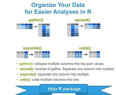
Here, you we’ll learn how to organize (or reshape) your data in order to make the analysis easier. This process is called tidying your data.


tibble data format: tbl_df
[Figure adapted from RStudio data wrangling cheatsheet (see reference section)]

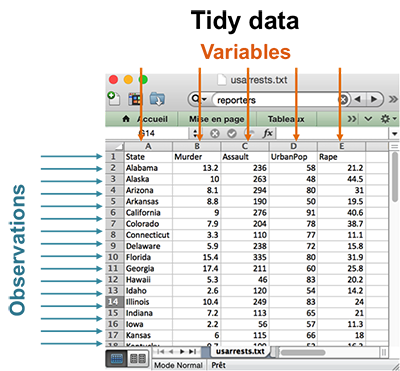
What is a tidy data set?

A data set is called tidy when:

  • each column represents a variable
  • and each row represents an observation

The opposite of tidy is messy data, which corresponds to any other arrangement of the data.

Tidy data

Having your data in tidy format is crucial for facilitating the tasks of data analysis including data manipulation, modeling and visualization.

The R package tidyr, developed by Hadley Wickham, provides functions to help you organize (or reshape) your data set into tidy format. It’s particularly designed to work in combination with magrittr and dplyr to build a solid data analysis pipeline.

Preleminary tasks

  1. Launch RStudio as described here: Running RStudio and setting up your working directory

  2. Import your data as described here: Importing data into R

Reshaping data using tidyr package

The tidyr package, provides four functions to help you change the layout of your data set:

  • gather(): gather (collapse) columns into rows
  • spread(): spread rows into columns
  • separate(): separate one column into multiple
  • unite(): unite multiple columns into one

Installing and loading tidyr

# Installing
install.packages("tidyr")

# Loading
library("tidyr")

Example data sets

We’ll use the R built-in USArrests data sets. We start by subsetting a small data set, which will be used in the next sections as an example data set:

my_data <- USArrests[c(1, 10, 20, 30), ]
my_data
           Murder Assault UrbanPop Rape
Alabama      13.2     236       58 21.2
Georgia      17.4     211       60 25.8
Maryland     11.3     300       67 27.8
New Jersey    7.4     159       89 18.8

Row names are states, so let’s use the function cbind() to add a column named “state” in the data. This will make the data tidy and the analysis easier.

my_data <- cbind(state = rownames(my_data), my_data)
my_data
                state Murder Assault UrbanPop Rape
Alabama       Alabama   13.2     236       58 21.2
Georgia       Georgia   17.4     211       60 25.8
Maryland     Maryland   11.3     300       67 27.8
New Jersey New Jersey    7.4     159       89 18.8

gather(): collapse columns into rows


The function gather() collapses multiple columns into key-value pairs. It produces a “long” data format from a “wide” one. It’s an alternative of melt() function [in reshape2 package].


tidyr gather

  1. Simplified format:
gather(data, key, value, ...)

  • data: A data frame
  • key, value: Names of key and value columns to create in output
  • …: Specification of columns to gather. Allowed values are:
    • variable names
    • if you want to select all variables between a and e, use a:e
    • if you want to exclude a column name y use -y
    • for more options, see: dplyr::select()


  1. Examples of usage:
  • Gather all columns except the column state
my_data2 <- gather(my_data,
                   key = "arrest_attribute",
                   value = "arrest_estimate",
                   -state)
my_data2
        state arrest_attribute arrest_estimate
1     Alabama           Murder            13.2
2     Georgia           Murder            17.4
3    Maryland           Murder            11.3
4  New Jersey           Murder             7.4
5     Alabama          Assault           236.0
6     Georgia          Assault           211.0
7    Maryland          Assault           300.0
8  New Jersey          Assault           159.0
9     Alabama         UrbanPop            58.0
10    Georgia         UrbanPop            60.0
11   Maryland         UrbanPop            67.0
12 New Jersey         UrbanPop            89.0
13    Alabama             Rape            21.2
14    Georgia             Rape            25.8
15   Maryland             Rape            27.8
16 New Jersey             Rape            18.8

Note that, all column names (except state) have been collapsed into a single key column (here “arrest_attribute”). Their values have been put into a value column (here “arrest_estimate”).

  • Gather only Murder and Assault columns
my_data2 <- gather(my_data,
                   key = "arrest_attribute",
                   value = "arrest_estimate",
                   Murder, Assault)
my_data2
       state UrbanPop Rape arrest_attribute arrest_estimate
1    Alabama       58 21.2           Murder            13.2
2    Georgia       60 25.8           Murder            17.4
3   Maryland       67 27.8           Murder            11.3
4 New Jersey       89 18.8           Murder             7.4
5    Alabama       58 21.2          Assault           236.0
6    Georgia       60 25.8          Assault           211.0
7   Maryland       67 27.8          Assault           300.0
8 New Jersey       89 18.8          Assault           159.0

Note that, the two columns Murder and Assault have been collapsed and the remaining columns (state, UrbanPop and Rape) have been duplicated.

  • Gather all variables between Murder and UrbanPop
my_data2 <- gather(my_data,
                   key = "arrest_attribute",
                   value = "arrest_estimate",
                   Murder:UrbanPop)
my_data2
        state Rape arrest_attribute arrest_estimate
1     Alabama 21.2           Murder            13.2
2     Georgia 25.8           Murder            17.4
3    Maryland 27.8           Murder            11.3
4  New Jersey 18.8           Murder             7.4
5     Alabama 21.2          Assault           236.0
6     Georgia 25.8          Assault           211.0
7    Maryland 27.8          Assault           300.0
8  New Jersey 18.8          Assault           159.0
9     Alabama 21.2         UrbanPop            58.0
10    Georgia 25.8         UrbanPop            60.0
11   Maryland 27.8         UrbanPop            67.0
12 New Jersey 18.8         UrbanPop            89.0

The remaining state column is duplicated.

  1. How to use gather() programmatically inside an R function?

You should use the function gather_() which takes character vectors, containing column names, instead of unquoted column names

The simplified syntax is as follow:

gather_(data, key_col, value_col, gather_cols)

  • data: a data frame
  • key_col, value_col: Strings specifying the names of key and value columns to create
  • gather_cols: Character vector specifying column names to be gathered together into pair of key-value columns.


As an example, type this:

gather_(my_data,
       key_col = "arrest_attribute",
       value_col = "arrest_estimate",
       gather_cols = c("Murder", "Assault"))

spread(): spread two columns into multiple columns


The function spread() does the reverse of gather(). It takes two columns (key and value) and spreads into multiple columns. It produces a “wide” data format from a “long” one. It’s an alternative of the function cast() [in reshape2 package].


tidyr spread

  1. Simplified format:
spread(data, key, value)

  • data: A data frame
  • key: The (unquoted) name of the column whose values will be used as column headings.
  • value:The (unquoted) names of the column whose values will populate the cells.


  1. Examples of usage:

Spread “my_data2” to turn back to the original data:

my_data3 <- spread(my_data2, 
                   key = "arrest_attribute",
                   value = "arrest_estimate"
                   )
my_data3
       state Rape Assault Murder UrbanPop
1    Alabama 21.2     236   13.2       58
2    Georgia 25.8     211   17.4       60
3   Maryland 27.8     300   11.3       67
4 New Jersey 18.8     159    7.4       89
  1. How to use spread() programmatically inside an R function?

You should use the function spread_() which takes strings specifying key and value columns instead of unquoted column names

The simplified syntax is as follow:

spread_(data, key_col, value_col)

  • data: a data frame.
  • key_col, value_col: Strings specifying the names of key and value columns.


As an example, type this:

spread_(my_data2, 
       key = "arrest_attribute",
       value = "arrest_estimate"
       )

unite(): Unite multiple columns into one


The function unite() takes multiple columns and paste them together into one.


tidyr unite

  1. Simplified format:
unite(data, col, ..., sep = "_")

  • data: A data frame
  • col: The new (unquoted) name of column to add.
  • sep: Separator to use between values


  1. Examples of usage:

The R code below uses the data set “my_data” and unites the columns Murder and Assault

my_data4 <- unite(my_data,
                  col = "Murder_Assault",
                  Murder, Assault,
                  sep = "_")
my_data4
                state Murder_Assault UrbanPop Rape
Alabama       Alabama       13.2_236       58 21.2
Georgia       Georgia       17.4_211       60 25.8
Maryland     Maryland       11.3_300       67 27.8
New Jersey New Jersey        7.4_159       89 18.8
  1. How to use unite() programmatically inside an R function?

You should use the function unite_() as follow.

unite_(data, col, from, sep = "_")

  • data: A data frame.
  • col: String giving the name of the new column to be added
  • from: Character vector specifying the names of existing columns to be united
  • sep: Separator to use between values.


As an example, type this:

unite_(my_data,
    col = "Murder_Assault",
    from = c("Murder", "Assault"),
    sep = "_")

separate(): separate one column into multiple


The function sperate() is the reverse of unite(). It takes values inside a single character column and separates them into multiple columns.


tidyr separate

  1. Simplified format:
separate(data, col, into, sep = "[^[:alnum:]]+")

  • data: A data frame
  • col: Unquoted column names
  • into: Character vector specifying the names of new variables to be created.
  • sep: Separator between columns:
    • If character, is interpreted as a regular expression.
    • If numeric, interpreted as positions to split at. Positive values start at 1 at the far-left of the string; negative value start at -1 at the far-right of the string.


  1. Examples of usage:

Separate the column “Murder_Assault” [in my_data4] into two columns Murder and Assault:

separate(my_data4,
         col = "Murder_Assault",
         into = c("Murder", "Assault"),
         sep = "_")
                state Murder Assault UrbanPop Rape
Alabama       Alabama   13.2     236       58 21.2
Georgia       Georgia   17.4     211       60 25.8
Maryland     Maryland   11.3     300       67 27.8
New Jersey New Jersey    7.4     159       89 18.8
  1. How to use separate() programmatically inside an R function?

You should use the function separate_() as follow.

separate_(data, col, into, sep = "[^[:alnum:]]+")

  • data: A data frame.
  • col: String giving the name of the column to split
  • into: Character vector specifying the names of new columns to create
  • sep: Separator between columns (as above).


As an example, type this:

separate_(my_data4,
         col = "Murder_Assault",
         into = c("Murder", "Assault"),
         sep = "_")

Chaining multiple operations

It’s possible to combine multiple operations using maggrittr forward-pipe operator : %>%.

For example, x %>% f is equivalent to f(x).

In the following R code:

  • first, my_data is passed to gather() function
  • next, the output of gather() is passed to unite() function
my_data %>% gather(key = "arrest_attribute",
                   value = "arrest_estimate",
                   Murder:UrbanPop) %>%
            unite(col = "attribute_estimate",
                  arrest_attribute, arrest_estimate)
        state Rape attribute_estimate
1     Alabama 21.2        Murder_13.2
2     Georgia 25.8        Murder_17.4
3    Maryland 27.8        Murder_11.3
4  New Jersey 18.8         Murder_7.4
5     Alabama 21.2        Assault_236
6     Georgia 25.8        Assault_211
7    Maryland 27.8        Assault_300
8  New Jersey 18.8        Assault_159
9     Alabama 21.2        UrbanPop_58
10    Georgia 25.8        UrbanPop_60
11   Maryland 27.8        UrbanPop_67
12 New Jersey 18.8        UrbanPop_89

Summary

You should tidy your data for easier data analysis using the R package tidyr, which provides the following functions.


  • Collapse multiple columns together into key-value pairs (long data format): gather(data, key, value, …)

  • Spread key-value pairs into multiple columns (wide data format): spread(data, key, value)

  • Unite multiple columns into one: unite(data, col, …)

  • Separate one columns into multiple: separate(data, col, into)


References

Infos

This analysis has been performed using R (ver. 3.2.3).

Reordering Data Frame Columns in R

$
0
0


Previously, we described the essentials of R programming and provided quick start guides for importing data into R as well as converting your data into a tibble data format, which is the best and modern way to work with your data. We also described crutial steps to reshape your data with R for easier analyses.


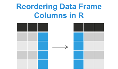
Here, you we’ll learn how to reorder columns, in your data table, by either column positions or column names.


Reordering Data Table Columns in R

Pleleminary tasks

  1. Launch RStudio as described here: Running RStudio and setting up your working directory

  2. Prepare your data as described here: Best practices for preparing your data and save it in an external .txt tab or .csv files

  3. Import your data into R as described here: Fast reading of data from txt|csv files into R: readr package.

Here, we’ll use the R built-in iris data set, which we start by converting to a tibble data frame (tbl_df). Tibble is a modern rethinking of data frame providing a nicer printing method. This is useful when working with large data sets.

# Create my_data
my_data <- iris

# Convert to a tibble
library("tibble")
my_data <- as_data_frame(my_data)

# Print
my_data
Source: local data frame [150 x 5]

   Sepal.Length Sepal.Width Petal.Length Petal.Width Species
          <dbl>       <dbl>        <dbl>       <dbl>  <fctr>
1           5.1         3.5          1.4         0.2  setosa
2           4.9         3.0          1.4         0.2  setosa
3           4.7         3.2          1.3         0.2  setosa
4           4.6         3.1          1.5         0.2  setosa
5           5.0         3.6          1.4         0.2  setosa
6           5.4         3.9          1.7         0.4  setosa
7           4.6         3.4          1.4         0.3  setosa
8           5.0         3.4          1.5         0.2  setosa
9           4.4         2.9          1.4         0.2  setosa
10          4.9         3.1          1.5         0.1  setosa
..          ...         ...          ...         ...     ...

Reorder column by position

# Get column names
colnames(my_data)
[1] "Sepal.Length" "Sepal.Width"  "Petal.Length" "Petal.Width"  "Species"     

my_data contains 5 columns ordered as follow:

  1. Sepal.Length
  2. Sepal.Width
  3. Petal.Length
  4. Petal.Width
  5. Species

But we want:

  • the variable “Species” to be the first column (1)
  • the variable “Petal.Width” to be the second column (2)

It’s possible to reorder the column by position as follow:

my_data2 <- my_data[, c(5, 4, 1, 2, 3)]
my_data2
Source: local data frame [150 x 5]

   Species Petal.Width Sepal.Length Sepal.Width Petal.Length
    <fctr>       <dbl>        <dbl>       <dbl>        <dbl>
1   setosa         0.2          5.1         3.5          1.4
2   setosa         0.2          4.9         3.0          1.4
3   setosa         0.2          4.7         3.2          1.3
4   setosa         0.2          4.6         3.1          1.5
5   setosa         0.2          5.0         3.6          1.4
6   setosa         0.4          5.4         3.9          1.7
7   setosa         0.3          4.6         3.4          1.4
8   setosa         0.2          5.0         3.4          1.5
9   setosa         0.2          4.4         2.9          1.4
10  setosa         0.1          4.9         3.1          1.5
..     ...         ...          ...         ...          ...

Reorder column by name

col_order <- c("Species", "Petal.Width", "Sepal.Length","Sepal.Width", "Petal.Length")

my_data2 <- my_data[, col_order]
my_data2
Source: local data frame [150 x 5]

   Species Petal.Width Sepal.Length Sepal.Width Petal.Length
    <fctr>       <dbl>        <dbl>       <dbl>        <dbl>
1   setosa         0.2          5.1         3.5          1.4
2   setosa         0.2          4.9         3.0          1.4
3   setosa         0.2          4.7         3.2          1.3
4   setosa         0.2          4.6         3.1          1.5
5   setosa         0.2          5.0         3.6          1.4
6   setosa         0.4          5.4         3.9          1.7
7   setosa         0.3          4.6         3.4          1.4
8   setosa         0.2          5.0         3.4          1.5
9   setosa         0.2          4.4         2.9          1.4
10  setosa         0.1          4.9         3.1          1.5
..     ...         ...          ...         ...          ...

Summary


It’s possible to reorder columns by either column position (i.e., number) or column names.


References

Infos

This analysis has been performed using R (ver. 3.2.3).

Reordering Data Frame Rows in R

$
0
0


Previously, we described the essentials of R programming and provided quick start guides for importing data into R as well as converting your data into a tibble data format, which is the best and modern way to work with your data. We also described crutial steps to reshape your data with R for easier analyses.


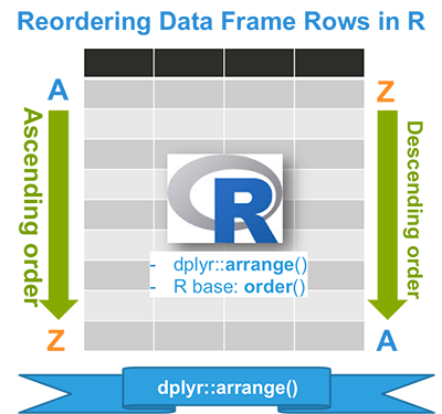
Here, you we’ll learn how to reorder (i.e., sort) rows, in your data table, by the value of one or more columns (i.e., variables). This can be done using either the R base function order() or the modern function arrange()[in dplyr package]. We recommend dplyr::arrange() because it requires less typing.


Reordering Data Frame Rows by Variables in R

Pleleminary tasks

  1. Launch RStudio as described here: Running RStudio and setting up your working directory

  2. Prepare your data as described here: Best practices for preparing your data and save it in an external .txt tab or .csv files

  3. Import your data into R as described here: Fast reading of data from txt|csv files into R: readr package.

Here, we’ll use the R built-in iris data set, which we start by converting to a tibble data frame (tbl_df). Tibble is a modern rethinking of data frame providing a nicer printing method. This is useful when working with large data sets.

# Create my_data
my_data <- iris

# Convert to a tibble
library("tibble")
my_data <- as_data_frame(my_data)

# Print
my_data
Source: local data frame [150 x 5]

   Sepal.Length Sepal.Width Petal.Length Petal.Width Species
          <dbl>       <dbl>        <dbl>       <dbl>  <fctr>
1           5.1         3.5          1.4         0.2  setosa
2           4.9         3.0          1.4         0.2  setosa
3           4.7         3.2          1.3         0.2  setosa
4           4.6         3.1          1.5         0.2  setosa
5           5.0         3.6          1.4         0.2  setosa
6           5.4         3.9          1.7         0.4  setosa
7           4.6         3.4          1.4         0.3  setosa
8           5.0         3.4          1.5         0.2  setosa
9           4.4         2.9          1.4         0.2  setosa
10          4.9         3.1          1.5         0.1  setosa
..          ...         ...          ...         ...     ...

Install and load dplyr package

  • Install dplyr
install.packages("dplyr")
  • Load dplyr:
library("dplyr")

Reorder rows with dplyr::arrange()


The dplyr function arrange() can be used to reorder (sort) rows by one or more variables.


  • Reorder rows by Sepal.Length in ascending order
arrange(my_data, Sepal.Length)
Source: local data frame [150 x 5]

   Sepal.Length Sepal.Width Petal.Length Petal.Width Species
          (dbl)       (dbl)        (dbl)       (dbl)  (fctr)
1           4.3         3.0          1.1         0.1  setosa
2           4.4         2.9          1.4         0.2  setosa
3           4.4         3.0          1.3         0.2  setosa
4           4.4         3.2          1.3         0.2  setosa
5           4.5         2.3          1.3         0.3  setosa
6           4.6         3.1          1.5         0.2  setosa
7           4.6         3.4          1.4         0.3  setosa
8           4.6         3.6          1.0         0.2  setosa
9           4.6         3.2          1.4         0.2  setosa
10          4.7         3.2          1.3         0.2  setosa
..          ...         ...          ...         ...     ...
  • Reorder rows by Sepal.Length in descending order. Use the function desc():
arrange(my_data, desc(Sepal.Length))
Source: local data frame [150 x 5]

   Sepal.Length Sepal.Width Petal.Length Petal.Width   Species
          (dbl)       (dbl)        (dbl)       (dbl)    (fctr)
1           7.9         3.8          6.4         2.0 virginica
2           7.7         3.8          6.7         2.2 virginica
3           7.7         2.6          6.9         2.3 virginica
4           7.7         2.8          6.7         2.0 virginica
5           7.7         3.0          6.1         2.3 virginica
6           7.6         3.0          6.6         2.1 virginica
7           7.4         2.8          6.1         1.9 virginica
8           7.3         2.9          6.3         1.8 virginica
9           7.2         3.6          6.1         2.5 virginica
10          7.2         3.2          6.0         1.8 virginica
..          ...         ...          ...         ...       ...

Instead of using the function desc(), you can prepend the sorting variable by a minus sign to indicate descending order, as follow.

arrange(my_data, -Sepal.Length)
  • Reorder rows by multiple variables: Sepal.Length and Sepal.width
arrange(my_data, Sepal.Length, Sepal.Width)
Source: local data frame [150 x 5]

   Sepal.Length Sepal.Width Petal.Length Petal.Width Species
          (dbl)       (dbl)        (dbl)       (dbl)  (fctr)
1           4.3         3.0          1.1         0.1  setosa
2           4.4         2.9          1.4         0.2  setosa
3           4.4         3.0          1.3         0.2  setosa
4           4.4         3.2          1.3         0.2  setosa
5           4.5         2.3          1.3         0.3  setosa
6           4.6         3.1          1.5         0.2  setosa
7           4.6         3.2          1.4         0.2  setosa
8           4.6         3.4          1.4         0.3  setosa
9           4.6         3.6          1.0         0.2  setosa
10          4.7         3.2          1.3         0.2  setosa
..          ...         ...          ...         ...     ...

If the data contain missing values, they will always come at the end.

dplyr::arrange() is the homologous of R base function order(). It requires less typing.

Reorder rows with R base function order()

  • Reorder rows by Sepal.Length in ascending order
my_data[order(my_data$Sepal.Length), , drop = FALSE]
  • Reorder rows by Sepal.Length in descending order. Use the additional argument decreasing = TRUE:
row_order <- order(my_data$Sepal.Length, decreasing = TRUE)
my_data[row_order, , drop = FALSE]

Summary


To order rows by values of a column use the function arrange()[in dplyr package].


Infos

This analysis has been performed using R (ver. 3.2.3).


Renaming Data Frame Columns in R

$
0
0


Previously, we described the essentials of R programming and provided quick start guides for importing data into R as well as converting your data into a tibble data format, which is the best and modern way to work with your data. We also described crutial steps to reshape your data with R for easier analyses.


Here, you we’ll learn how to rename the columns of a data frame in R.This can be done easily using the function rename() in dplyr. It’s also possible to use R base functions, but they require more typing.


Renaming Columns of a Data Table in R

Pleleminary tasks

  1. Launch RStudio as described here: Running RStudio and setting up your working directory

  2. Prepare your data as described here: Best practices for preparing your data and save it in an external .txt tab or .csv files

  3. Import your data into R as described here: Fast reading of data from txt|csv files into R: readr package.

Here, we’ll use the R built-in iris data set, which we start by converting to a tibble data frame (tbl_df). Tibble is a modern rethinking of data frame providing a nicer printing method. This is useful when working with large data sets.

# Create my_data
my_data <- iris

# Convert to a tibble
library("tibble")
my_data <- as_data_frame(my_data)

# Print
my_data
Source: local data frame [150 x 5]

   Sepal.Length Sepal.Width Petal.Length Petal.Width Species
          <dbl>       <dbl>        <dbl>       <dbl>  <fctr>
1           5.1         3.5          1.4         0.2  setosa
2           4.9         3.0          1.4         0.2  setosa
3           4.7         3.2          1.3         0.2  setosa
4           4.6         3.1          1.5         0.2  setosa
5           5.0         3.6          1.4         0.2  setosa
6           5.4         3.9          1.7         0.4  setosa
7           4.6         3.4          1.4         0.3  setosa
8           5.0         3.4          1.5         0.2  setosa
9           4.4         2.9          1.4         0.2  setosa
10          4.9         3.1          1.5         0.1  setosa
..          ...         ...          ...         ...     ...

Install and load dplyr package for renaming columns

  • Install dplyr
install.packages("dplyr")
  • Load dplyr:
library("dplyr")

Renaming columns with dplyr::rename()

  • Rename the column Sepal.Length to sepal_length and Sepal.Width to sepal_width:
rename(my_data, sepal_length = Sepal.Length,
       sepal_width = Sepal.Width)
Source: local data frame [150 x 5]

   sepal_length sepal_width Petal.Length Petal.Width Species
          (dbl)       (dbl)        (dbl)       (dbl)  (fctr)
1           5.1         3.5          1.4         0.2  setosa
2           4.9         3.0          1.4         0.2  setosa
3           4.7         3.2          1.3         0.2  setosa
4           4.6         3.1          1.5         0.2  setosa
5           5.0         3.6          1.4         0.2  setosa
6           5.4         3.9          1.7         0.4  setosa
7           4.6         3.4          1.4         0.3  setosa
8           5.0         3.4          1.5         0.2  setosa
9           4.4         2.9          1.4         0.2  setosa
10          4.9         3.1          1.5         0.1  setosa
..          ...         ...          ...         ...     ...

Renaming columns with dplyr::select()

select() can be also used to rename variables as follow.

select(my_data, sepal_length = Sepal.Length,
       sepal_width = Sepal.Width)
Source: local data frame [150 x 2]

   sepal_length sepal_width
          (dbl)       (dbl)
1           5.1         3.5
2           4.9         3.0
3           4.7         3.2
4           4.6         3.1
5           5.0         3.6
6           5.4         3.9
7           4.6         3.4
8           5.0         3.4
9           4.4         2.9
10          4.9         3.1
..          ...         ...

Note that, select() keeps only the variables you mentioned. In order to to keep all, you can use the function rename(), which is an alternative of select().

Renaming columns with R base functions

To rename the column Sepal.Length to sepal_length, the procedure is as follow:

  1. Get column names using the function names() or colnames()
  2. Change column names where name = Sepal.Length
# get column names
colnames(my_data)
[1] "Sepal.Length" "Sepal.Width"  "Petal.Length" "Petal.Width"  "Species"     
# Rename column where names is "Sepal.Length"
names(my_data)[names(my_data) == "Sepal.Length"] <- "sepal_length"
names(my_data)[names(my_data) == "Sepal.Width"] <- "sepal_width"
my_data
Source: local data frame [150 x 5]

   sepal_length sepal_width Petal.Length Petal.Width Species
          (dbl)       (dbl)        (dbl)       (dbl)  (fctr)
1           5.1         3.5          1.4         0.2  setosa
2           4.9         3.0          1.4         0.2  setosa
3           4.7         3.2          1.3         0.2  setosa
4           4.6         3.1          1.5         0.2  setosa
5           5.0         3.6          1.4         0.2  setosa
6           5.4         3.9          1.7         0.4  setosa
7           4.6         3.4          1.4         0.3  setosa
8           5.0         3.4          1.5         0.2  setosa
9           4.4         2.9          1.4         0.2  setosa
10          4.9         3.1          1.5         0.1  setosa
..          ...         ...          ...         ...     ...

It’s also possible to rename by index in names vector as follow.

names(my_data)[1] <- "sepal_length"
names(my_data)[2] <- "sepal_width"

Summary


To rename the column of a data frame, use the function rename()[in dplyr package].


Infos

This analysis has been performed using R (ver. 3.2.3).

Subsetting Data Frame Rows in R

$
0
0


Previously, we described the essentials of R programming and provided quick start guides for importing data into R as well as converting your data into a tibble data format, which is the best and modern way to work with your data. We also described crutial steps to reshape your data with R for easier analyses.


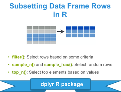
Here, you we’ll learn how to subset (or filter) rows of a data frame based on certain criteria. This can be done easily using R functions provided by dplyr package. It’s also possible to use the R base functions subset().


Among the functions available in dplyr package, there are:

  • filter(iris, Sepal.Length >7): Extract rows based on logical criteria
  • distinct(iris): Remove duplicated rows
  • sample_n(iris, 10, replace = FALSE): Select n random rows from a table
  • sample_frac(iris, 0.5, replace = FALSE): Select a random fraction of rows
  • slice(iris, 3:8): Select rows by position
  • top_n(iris, 10, Sepal.Length): Select and order top n rows (by groups if grouped data)

We’ll start by describing how to subset rows based on some criteria, with the dplyr::filter() function as well as the R base function subset(). Next, we’ll show you how to select rows randomly using sample_n() and sample_frac() functions. Finally, we’ll describe how to select the top n elements in each group, ordered by a given variables.

Subsetting Data Frame Rows in R

Pleleminary tasks

  1. Launch RStudio as described here: Running RStudio and setting up your working directory

  2. Prepare your data as described here: Best practices for preparing your data and save it in an external .txt tab or .csv files

  3. Import your data into R as described here: Fast reading of data from txt|csv files into R: readr package.

Here, we’ll use the R built-in iris data set, which we start by converting to a tibble data frame (tbl_df). Tibble is a modern rethinking of data frame providing a nicer printing method. This is useful when working with large data sets.

# Create my_data
my_data <- iris

# Convert to a tibble
library("tibble")
my_data <- as_data_frame(my_data)

# Print
my_data
Source: local data frame [150 x 5]

   Sepal.Length Sepal.Width Petal.Length Petal.Width Species
          <dbl>       <dbl>        <dbl>       <dbl>  <fctr>
1           5.1         3.5          1.4         0.2  setosa
2           4.9         3.0          1.4         0.2  setosa
3           4.7         3.2          1.3         0.2  setosa
4           4.6         3.1          1.5         0.2  setosa
5           5.0         3.6          1.4         0.2  setosa
6           5.4         3.9          1.7         0.4  setosa
7           4.6         3.4          1.4         0.3  setosa
8           5.0         3.4          1.5         0.2  setosa
9           4.4         2.9          1.4         0.2  setosa
10          4.9         3.1          1.5         0.1  setosa
..          ...         ...          ...         ...     ...

Install and load dplyr package

  • Install dplyr
install.packages("dplyr")
  • Load dplyr:
library("dplyr")

Extracting rows by position: dplyr::slice()

Select rows 1 to 6:

my_data[1:6, ]

or you can also use the function slice()[in dplyr]:

slice(my_data, 1:6)

Extracting rows by criteria: dplyr::filter()


The function filter() is used to filter rows that meet some logical criteria.


Logical comparisons

Before continuing, we introduce the notion of logical comparisons and operators, which are important to know for filtering data.

The “logical” comparison operators available in R are:


  1. Logical comparisons
    • <: for less than
    • >: for greater than
    • <=: for less than or equal to
    • >=: for greater than or equal to
    • ==: for equal to each other
    • !=: not equal to each other
    • %in%: group membership. For example, “value %in% c(2, 3)” means that value can takes 2 or 3.
    • is.na(): is NA
    • !is.na(): is not NA.
  2. Logical operators
    • value == 2|3: means that the value equal 2 or (|) 3. value %in% c(2, 3) is a shortcut equivalent to value == 2|3.
    • &: means and. For example sex == “female” & age > 25


The most frequent mistake made by beginners in R is to use = instead of == when testing for equality. Remember that, when you are testing for equality, you should always use == (not =).

Extracting rows based on logical criteria

  • One-column based criteria: Extract rows where Sepal.Length > 7:
filter(my_data, Sepal.Length > 7)
Source: local data frame [12 x 5]

   Sepal.Length Sepal.Width Petal.Length Petal.Width   Species
          (dbl)       (dbl)        (dbl)       (dbl)    (fctr)
1           7.1         3.0          5.9         2.1 virginica
2           7.6         3.0          6.6         2.1 virginica
3           7.3         2.9          6.3         1.8 virginica
4           7.2         3.6          6.1         2.5 virginica
5           7.7         3.8          6.7         2.2 virginica
6           7.7         2.6          6.9         2.3 virginica
7           7.7         2.8          6.7         2.0 virginica
8           7.2         3.2          6.0         1.8 virginica
9           7.2         3.0          5.8         1.6 virginica
10          7.4         2.8          6.1         1.9 virginica
11          7.9         3.8          6.4         2.0 virginica
12          7.7         3.0          6.1         2.3 virginica
  • Multiple-column based criteria: Extract rows where Sepal.Length > 6.7 and Sepal.Width ≤ 3:
filter(my_data, Sepal.Length > 6.7, Sepal.Width <= 3)
Source: local data frame [10 x 5]

   Sepal.Length Sepal.Width Petal.Length Petal.Width    Species
          (dbl)       (dbl)        (dbl)       (dbl)     (fctr)
1           6.8         2.8          4.8         1.4 versicolor
2           7.1         3.0          5.9         2.1  virginica
3           7.6         3.0          6.6         2.1  virginica
4           7.3         2.9          6.3         1.8  virginica
5           6.8         3.0          5.5         2.1  virginica
6           7.7         2.6          6.9         2.3  virginica
7           7.7         2.8          6.7         2.0  virginica
8           7.2         3.0          5.8         1.6  virginica
9           7.4         2.8          6.1         1.9  virginica
10          7.7         3.0          6.1         2.3  virginica
  • Test for equality (==): Extract rows where Sepal.Length > 6.5 and Species = “versicolor”:
filter(my_data, Sepal.Length > 6.7, Species == "versicolor")
Source: local data frame [3 x 5]

  Sepal.Length Sepal.Width Petal.Length Petal.Width    Species
         (dbl)       (dbl)        (dbl)       (dbl)     (fctr)
1          7.0         3.2          4.7         1.4 versicolor
2          6.9         3.1          4.9         1.5 versicolor
3          6.8         2.8          4.8         1.4 versicolor
  • Using OR operator (|): Extract rows where Sepal.Length > 6.5 and (Species = “versicolor” or Species = “virginica”):

Use this:

filter(my_data, Sepal.Length > 6.7, 
       Species == "versicolor" | Species == "virginica" )

Or, equivalently, use this shortcut (%in% operator):

filter(my_data, Sepal.Length > 6.7, 
      Species %in% c("versicolor", "virginica" ))
Source: local data frame [20 x 5]

   Sepal.Length Sepal.Width Petal.Length Petal.Width    Species
          (dbl)       (dbl)        (dbl)       (dbl)     (fctr)
1           7.0         3.2          4.7         1.4 versicolor
2           6.9         3.1          4.9         1.5 versicolor
3           6.8         2.8          4.8         1.4 versicolor
4           7.1         3.0          5.9         2.1  virginica
5           7.6         3.0          6.6         2.1  virginica
6           7.3         2.9          6.3         1.8  virginica
7           7.2         3.6          6.1         2.5  virginica
8           6.8         3.0          5.5         2.1  virginica
9           7.7         3.8          6.7         2.2  virginica
10          7.7         2.6          6.9         2.3  virginica
11          6.9         3.2          5.7         2.3  virginica
12          7.7         2.8          6.7         2.0  virginica
13          7.2         3.2          6.0         1.8  virginica
14          7.2         3.0          5.8         1.6  virginica
15          7.4         2.8          6.1         1.9  virginica
16          7.9         3.8          6.4         2.0  virginica
17          7.7         3.0          6.1         2.3  virginica
18          6.9         3.1          5.4         2.1  virginica
19          6.9         3.1          5.1         2.3  virginica
20          6.8         3.2          5.9         2.3  virginica

Note that, filter() works similarly to the R base function subset(), which will be described in the next sections.

Removing missing values

As described in the chapter named R programming basics, it’s possible to use the function is.na(x) to check whether a data contains missing value. It takes a vector x as an input and returns a logical vector in which the value TRUE specifies that the corresponding element in x is NA.

  • Create a tbl with missing values using data_frame() [in dplyr]. In R NA (Not Available) is used to represent missing values:
# Create a data frame with missing data
friends_data <- data_frame(
  name = c("Nicolas", "Thierry", "Bernard", "Jerome"),
  age = c(27, 25, 29, 26),
  height = c(180, NA, NA, 169),
  married = c("yes", "yes", "no", "no")
)
# Print
friends_data
Source: local data frame [4 x 4]

     name   age height married
    (chr) (dbl)  (dbl)   (chr)
1 Nicolas    27    180     yes
2 Thierry    25     NA     yes
3 Bernard    29     NA      no
4  Jerome    26    169      no
  • Extract rows where height is NA:
filter(friends_data, is.na(height))
Source: local data frame [2 x 4]

     name   age height married
    (chr) (dbl)  (dbl)   (chr)
1 Thierry    25     NA     yes
2 Bernard    29     NA      no
  • Exclude (drop) rows where height is NA:
filter(friends_data, !is.na(height))
Source: local data frame [2 x 4]

     name   age height married
    (chr) (dbl)  (dbl)   (chr)
1 Nicolas    27    180     yes
2  Jerome    26    169      no

In the R code above, !is.na() means that “we don’t want” NAs.

Using filter() programmatically inside an R function


filter() is best-suited for interactive use. The function filter_() should be used for calling from a function. In this case the input must be “quoted”.


There are three ways to quote inputs that dplyr understands:

  • With a formula, ~Sepal.Length.
  • With quote(), quote(Sepal.Length).
  • As a string: “Sepal.Length”.
# Extract rows where Sepal.Length > 7
filter_(my_data, "Sepal.Length > 7")

# Extract rows where Sepal.Length > 7 and Sepal.Width <= 3
filter_(my_data, "Sepal.Length > 7 & Sepal.Width <= 3")

# Extract rows where Sepal.Length > 6.5 and
# (Species = "versicolor" or Species = "virginica")
filter_(my_data, quote(Sepal.Length > 6.7 & 
      Species %in% c("versicolor", "virginica" )))

Extracting rows by criteria with R base functions: subset()

  • Extract rows where Sepal.Length > 7 and Sepal.Width ≤ 3:

You can use this:

my_data[my_data$Sepal.Length > 7 & my_data$Sepal.Width <= 3, ]

Or use the R base function subset():

subset(my_data, Sepal.Length > 7 & Sepal.Width <= 3)
  • Extract rows where Sepal.Length > 6.7 and (Species = “versicolor” or Species = “virginica”)
subset(my_data, Sepal.Length > 6.7, 
      Species %in% c("versicolor", "virginica" ))

subset() works also with vectors as follow.

my_vec <- 1:10
subset(my_vec, my_vec >5 & my_vec < 8)
[1] 6 7

Note that, R base functions require more typing than dplyr::filter(), so we recommend dplyr solutions.

Select random rows from a table


It’s possible to select either n random rows with the function sample_n() or a random fraction of rows with sample_frac().


We first use the function set.seed() to initiate random number generator engine. This important for users to reproduce the analysis.

set.seed(1234)
# Extract 5 random rows without replacement
sample_n(my_data, 5, replace = FALSE)
Source: local data frame [5 x 5]

  Sepal.Length Sepal.Width Petal.Length Petal.Width    Species
         (dbl)       (dbl)        (dbl)       (dbl)     (fctr)
1          5.1         3.5          1.4         0.3     setosa
2          5.8         2.6          4.0         1.2 versicolor
3          5.5         2.6          4.4         1.2 versicolor
4          6.1         3.0          4.6         1.4 versicolor
5          7.2         3.2          6.0         1.8  virginica
# Extract 5% of rows, randomly without replacement
sample_frac(my_data, 0.05, replace = FALSE)
Source: local data frame [8 x 5]

  Sepal.Length Sepal.Width Petal.Length Petal.Width    Species
         (dbl)       (dbl)        (dbl)       (dbl)     (fctr)
1          5.7         2.9          4.2         1.3 versicolor
2          4.9         3.0          1.4         0.2     setosa
3          4.9         3.1          1.5         0.2     setosa
4          6.2         2.9          4.3         1.3 versicolor
5          6.6         3.0          4.4         1.4 versicolor
6          6.3         3.3          6.0         2.5  virginica
7          6.0         2.9          4.5         1.5 versicolor
8          5.0         3.5          1.3         0.3     setosa

Note that, it’s also possible to use the R base function sample(), but it requires more typing.

set.seed(1234)
my_data[sample(1:nrow(my_data), 5, replace = FALSE), , drop = FALSE]

Select top n rows ordered by a variable


As mentioned above, the function top_n(), can be used to select the top n entries in each group.


  • The format is as follow:
top_n(x, n, wt)

  • x: Data table
  • n: Number of rows to return. If x is grouped, this is the number of rows per group. May include more than n if there are ties.
  • wt(Optional): The variable to use for ordering. If not specified, defaults to the last variable in the data table.


  • Select the top 5 rows ordered by Sepal.Length
top_n(my_data, 5, Sepal.Length)
Source: local data frame [5 x 5]

  Sepal.Length Sepal.Width Petal.Length Petal.Width   Species
         (dbl)       (dbl)        (dbl)       (dbl)    (fctr)
1          7.7         3.8          6.7         2.2 virginica
2          7.7         2.6          6.9         2.3 virginica
3          7.7         2.8          6.7         2.0 virginica
4          7.9         3.8          6.4         2.0 virginica
5          7.7         3.0          6.1         2.3 virginica
  • Group by the column Species and select the top 5 of each group ordered by Sepal.Length:
my_data %>% 
  group_by(Species) %>%
  top_n(5, Sepal.Length)

Note that, dplyr package allows to use the forward-pipe operator (%>%) for combining multiple operations. For example, x %>% f is equivalent to f(x). The output of each operation is passed to the next operation.

Summary


  • Filter rows by logical criteria: dplyr::filter(iris, Sepal.Length >7)

  • Select n random rows: dplyr::sample_n(iris, 10)

  • Select a random fraction of rows: dplyr::sample_frac(iris, 10)

  • Select top n rows by values: dplyr::top_n(iris, 10, Sepal.Length)


Infos

This analysis has been performed using R (ver. 3.2.3).

Subsetting Data Frame Columns in R

$
0
0


Previously, we described the essentials of R programming and provided quick start guides for importing data into R as well as converting your data into a tibble data format, which is the best and modern way to work with your data. We next described crutial steps to reshape your data with R for easier analyses. Additionally, we provided quick start guides for subsetting data frame rows based on some logical criteria.


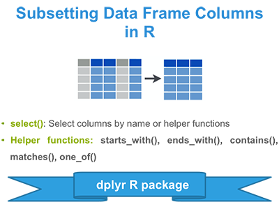
Here, you we’ll learn how to subset data frame columns (i.e., variables) by names using the function select() [in dplyr package].


Subsetting Columns of a Data Frame in R

Pleleminary tasks

  1. Launch RStudio as described here: Running RStudio and setting up your working directory

  2. Prepare your data as described here: Best practices for preparing your data and save it in an external .txt tab or .csv files

  3. Import your data into R as described here: Fast reading of data from txt|csv files into R: readr package.

Here, we’ll use the R built-in iris data set, which we start by converting to a tibble data frame (tbl_df). Tibble is a modern rethinking of data frame providing a nicer printing method. This is useful when working with large data sets.

# Create my_data
my_data <- iris

# Convert to a tibble
library("tibble")
my_data <- as_data_frame(my_data)

# Print
my_data
Source: local data frame [150 x 5]

   Sepal.Length Sepal.Width Petal.Length Petal.Width Species
          <dbl>       <dbl>        <dbl>       <dbl>  <fctr>
1           5.1         3.5          1.4         0.2  setosa
2           4.9         3.0          1.4         0.2  setosa
3           4.7         3.2          1.3         0.2  setosa
4           4.6         3.1          1.5         0.2  setosa
5           5.0         3.6          1.4         0.2  setosa
6           5.4         3.9          1.7         0.4  setosa
7           4.6         3.4          1.4         0.3  setosa
8           5.0         3.4          1.5         0.2  setosa
9           4.4         2.9          1.4         0.2  setosa
10          4.9         3.1          1.5         0.1  setosa
..          ...         ...          ...         ...     ...

Install and load dplyr package

  • Install dplyr
install.packages("dplyr")
  • Load dplyr:
library("dplyr")

Selecting column by position

  • Select columns 1 to 2:
my_data[, 1:2]
  • Select column 1 and 3 but not 2:
my_data[, c(1, 3)]

Select columns by names

  • Select columns by names: Sepal.Length and Petal.Length
select(my_data, Sepal.Length, Petal.Length)
Source: local data frame [150 x 2]

   Sepal.Length Petal.Length
          (dbl)        (dbl)
1           5.1          1.4
2           4.9          1.4
3           4.7          1.3
4           4.6          1.5
5           5.0          1.4
6           5.4          1.7
7           4.6          1.4
8           5.0          1.5
9           4.4          1.4
10          4.9          1.5
..          ...          ...
  • Select all columns from Sepal.Length to Petal.Length
select(my_data, Sepal.Length:Petal.Length)
Source: local data frame [150 x 3]

   Sepal.Length Sepal.Width Petal.Length
          (dbl)       (dbl)        (dbl)
1           5.1         3.5          1.4
2           4.9         3.0          1.4
3           4.7         3.2          1.3
4           4.6         3.1          1.5
5           5.0         3.6          1.4
6           5.4         3.9          1.7
7           4.6         3.4          1.4
8           5.0         3.4          1.5
9           4.4         2.9          1.4
10          4.9         3.1          1.5
..          ...         ...          ...

There are several special functions that can be used inside select(): starts_with(), ends_with(), contains(), matches(), one_of(), etc.

# Select column whose name starts with "Petal"
select(my_data, starts_with("Petal"))

# Select column whose name ends with "Width"
select(my_data, ends_with("Width"))

# Select columns whose names contains "etal"
select(my_data, contains("etal"))
# Select columns whose name maches a regular expression
select(my_data, matches(".t."))

# selects variables provided in a character vector.
select(my_data, one_of(c("Sepal.Length", "Petal.Length")))

Drop columns

Note that, to remove a column from a data frame, prepend its name by minus -.

  • Dropping Sepal.Length and Petal.Length:
select(my_data, -Sepal.Length, -Petal.Length)
  • Dropping columns from Sepal.Length to Petal.Length:
select(my_data, -(Sepal.Length:Petal.Length))
Source: local data frame [150 x 2]

   Petal.Width Species
         (dbl)  (fctr)
1          0.2  setosa
2          0.2  setosa
3          0.2  setosa
4          0.2  setosa
5          0.2  setosa
6          0.4  setosa
7          0.3  setosa
8          0.2  setosa
9          0.2  setosa
10         0.1  setosa
..         ...     ...
  • Dropping columns whose name starts with “Petal”:
select(my_data, -starts_with("Petal"))
Source: local data frame [150 x 3]

   Sepal.Length Sepal.Width Species
          (dbl)       (dbl)  (fctr)
1           5.1         3.5  setosa
2           4.9         3.0  setosa
3           4.7         3.2  setosa
4           4.6         3.1  setosa
5           5.0         3.6  setosa
6           5.4         3.9  setosa
7           4.6         3.4  setosa
8           5.0         3.4  setosa
9           4.4         2.9  setosa
10          4.9         3.1  setosa
..          ...         ...     ...

Note that, if you want to drop columns by position, the syntax is as follow.

# Drop column 1
my_data[, -1]

# Drop columns 1 to 3
my_data[, -(1:3)]

# Drop columns 1 and 3 but not 2
my_data[, -c(1, 3)]

Use select() programmatically inside an R function

Dplyr uses non-standard evaluation (NSE), which is great for interactive use and save you typing. Behind the scene, NSE is powered by the lazyeval package.


select() is best-suited for interactive use. The function select_() should be used for calling from a function. In this case the input must be “quoted”.


There are three ways to quote inputs that dplyr understands:

  • With a formula, ~Sepal.Length.
  • With quote(), quote(Sepal.Length).
  • As a string: “Sepal.Length”.

For example, you can select the column Sepal.Length by typing the following R code:

select_(my_data, ~Sepal.Length)

Or, by using this:

select_(my_data, "Sepal.Length")

It’s also possible to use function inside select_(). The R package lazyeval is required. It can be installed as follow:

install.packages("lazyeval")

Use lazyeval package to interpret functions inside select_():

# Select column names that match ".t."
select_(my_data, lazyeval::interp(~matches(x), x = ".t."))

# Select column names that start with "Petal"
select_(my_data, lazyeval::interp(~starts_with(x), x = "Petal"))

# Dropping columns: Sepal.Length and Sepal.Width
select_(my_data, quote(-Sepal.Length), quote(-Sepal.Width))

# Or use this
select_(my_data, .dots = list(quote(-Petal.Length), quote(-Petal.Width)))

Summary


  • Select columns by position: my_data[, 1:2]

  • Select columns by name: dplyr::select(my_data, Sepal.Length, Petal.Length)

  • Drop columns: dplyr::select(my_data, -Sepal.Length, -Petal.Length)

  • Helper functions: starts_with(), ends_with(), contains(), matches(), one_of()
    • dplyr::select(my_data, starts_with(“Petal”))
    • dplyr::select(my_data, ends_with(“Length”))


Infos

This analysis has been performed using R (ver. 3.2.3).

Identifying and Removing Duplicate Data in R

$
0
0


Previously, we described the essentials of R programming and provided quick start guides for importing data into R as well as converting your data into a tibble data format, which is the best and modern way to work with your data.


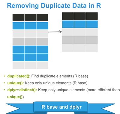
Here, you we’ll learn how to remove duplicate data using R base functions (duplicated() and unique()) as well as the function distinct [in dplyr package].


Identifying and Removing Duplicate Data in R

Pleleminary tasks

  1. Launch RStudio as described here: Running RStudio and setting up your working directory

  2. Prepare your data as described here: Best practices for preparing your data and save it in an external .txt tab or .csv files

  3. Import your data into R as described here: Fast reading of data from txt|csv files into R: readr package.

Here, we’ll use the R built-in iris data set, which we start by converting to a tibble data frame (tbl_df). Tibble is a modern rethinking of data frame providing a nicer printing method. This is useful when working with large data sets.

# Create my_data
my_data <- iris

# Convert to a tibble
library("tibble")
my_data <- as_data_frame(my_data)

# Print
my_data
Source: local data frame [150 x 5]

   Sepal.Length Sepal.Width Petal.Length Petal.Width Species
          <dbl>       <dbl>        <dbl>       <dbl>  <fctr>
1           5.1         3.5          1.4         0.2  setosa
2           4.9         3.0          1.4         0.2  setosa
3           4.7         3.2          1.3         0.2  setosa
4           4.6         3.1          1.5         0.2  setosa
5           5.0         3.6          1.4         0.2  setosa
6           5.4         3.9          1.7         0.4  setosa
7           4.6         3.4          1.4         0.3  setosa
8           5.0         3.4          1.5         0.2  setosa
9           4.4         2.9          1.4         0.2  setosa
10          4.9         3.1          1.5         0.1  setosa
..          ...         ...          ...         ...     ...

R base functions


In this section, we’ll describe the function unique() [for extracting unique elements] and the function duplicated() [for identifying duplicated elements].


Find and drop duplicate elements: duplicated()

The function duplicated() returns a logical vector where TRUE specifies which elements of a vector or data frame are duplicates.

Given the following vector:

x <- c(1, 1, 4, 5, 4, 6)
  • To find the position of duplicate elements in x, use this:
duplicated(x)
[1] FALSE  TRUE FALSE FALSE  TRUE FALSE
  • Extract duplicate elements:
x[duplicated(x)]
[1] 1 4
  • If you want to remove duplicated elements, use !duplicated(), where ! is a logical negation:
x[!duplicated(x)]
[1] 1 4 5 6
  • Following this way, you can remove duplicate rows from a data frame based on a column values, as follow:
# Remove duplicates based on Sepal.Width columns
my_data[!duplicated(my_data$Sepal.Width), ]
Source: local data frame [23 x 5]

   Sepal.Length Sepal.Width Petal.Length Petal.Width Species
          <dbl>       <dbl>        <dbl>       <dbl>  <fctr>
1           5.1         3.5          1.4         0.2  setosa
2           4.9         3.0          1.4         0.2  setosa
3           4.7         3.2          1.3         0.2  setosa
4           4.6         3.1          1.5         0.2  setosa
5           5.0         3.6          1.4         0.2  setosa
6           5.4         3.9          1.7         0.4  setosa
7           4.6         3.4          1.4         0.3  setosa
8           4.4         2.9          1.4         0.2  setosa
9           5.4         3.7          1.5         0.2  setosa
10          5.8         4.0          1.2         0.2  setosa
..          ...         ...          ...         ...     ...

! is a logical negation. !duplicated() means that we don’t want duplicate rows.

Extract unique elements: unique()

Given the following vector:

x <- c(1, 1, 4, 5, 4, 6)

You can extract unique elements as follow:

unique(x)
[1] 1 4 5 6

It’s also possible to apply unique() on a data frame, for removing duplicated rows as follow:

unique(my_data)
Source: local data frame [149 x 5]

   Sepal.Length Sepal.Width Petal.Length Petal.Width Species
          <dbl>       <dbl>        <dbl>       <dbl>  <fctr>
1           5.1         3.5          1.4         0.2  setosa
2           4.9         3.0          1.4         0.2  setosa
3           4.7         3.2          1.3         0.2  setosa
4           4.6         3.1          1.5         0.2  setosa
5           5.0         3.6          1.4         0.2  setosa
6           5.4         3.9          1.7         0.4  setosa
7           4.6         3.4          1.4         0.3  setosa
8           5.0         3.4          1.5         0.2  setosa
9           4.4         2.9          1.4         0.2  setosa
10          4.9         3.1          1.5         0.1  setosa
..          ...         ...          ...         ...     ...

Remove duplicate rows using dplyr


The function distinct() in dplyr package can be used to keep only unique/distinct rows from a data frame. If there are duplicate rows, only the first row is preserved. It’s an efficient version of the R base function unique().


The dplyr package can be loaded and installed as follow:

# Install
install.packages("dplyr")

# Load
library("dplyr")
  • Remove duplicate rows based on all columns:
distinct(my_data)
Source: local data frame [149 x 5]

   Sepal.Length Sepal.Width Petal.Length Petal.Width Species
          (dbl)       (dbl)        (dbl)       (dbl)  (fctr)
1           5.1         3.5          1.4         0.2  setosa
2           4.9         3.0          1.4         0.2  setosa
3           4.7         3.2          1.3         0.2  setosa
4           4.6         3.1          1.5         0.2  setosa
5           5.0         3.6          1.4         0.2  setosa
6           5.4         3.9          1.7         0.4  setosa
7           4.6         3.4          1.4         0.3  setosa
8           5.0         3.4          1.5         0.2  setosa
9           4.4         2.9          1.4         0.2  setosa
10          4.9         3.1          1.5         0.1  setosa
..          ...         ...          ...         ...     ...
  • Remove duplicate rows based on certain columns (variables):
# Remove duplicated rows based on Sepal.Length
distinct(my_data, Sepal.Length)
Source: local data frame [35 x 5]

   Sepal.Length Sepal.Width Petal.Length Petal.Width Species
          (dbl)       (dbl)        (dbl)       (dbl)  (fctr)
1           5.1         3.5          1.4         0.2  setosa
2           4.9         3.0          1.4         0.2  setosa
3           4.7         3.2          1.3         0.2  setosa
4           4.6         3.1          1.5         0.2  setosa
5           5.0         3.6          1.4         0.2  setosa
6           5.4         3.9          1.7         0.4  setosa
7           4.4         2.9          1.4         0.2  setosa
8           4.8         3.4          1.6         0.2  setosa
9           4.3         3.0          1.1         0.1  setosa
10          5.8         4.0          1.2         0.2  setosa
..          ...         ...          ...         ...     ...
# Remove duplicated rows based on 
# Sepal.Length and Petal.Width
distinct(my_data, Sepal.Length, Petal.Width)
Source: local data frame [110 x 5]

   Sepal.Length Sepal.Width Petal.Length Petal.Width Species
          (dbl)       (dbl)        (dbl)       (dbl)  (fctr)
1           5.1         3.5          1.4         0.2  setosa
2           4.9         3.0          1.4         0.2  setosa
3           4.7         3.2          1.3         0.2  setosa
4           4.6         3.1          1.5         0.2  setosa
5           5.0         3.6          1.4         0.2  setosa
6           5.4         3.9          1.7         0.4  setosa
7           4.6         3.4          1.4         0.3  setosa
8           4.4         2.9          1.4         0.2  setosa
9           4.9         3.1          1.5         0.1  setosa
10          5.4         3.7          1.5         0.2  setosa
..          ...         ...          ...         ...     ...

distinct() is best-suited for interactive use. The function distinct_() should be used for calling from a function. In this case the input must be “quoted”.


distinct_(my_data,  "Sepal.Length", "Petal.Width")

Summary


  • Remove duplicate rows based on one or more column values: dplyr::distinct(my_data, Sepal.Length)

  • R base function to extract unique elements from vectors and data frames: unique(my_data)

  • R base function to determine duplicate elements: duplicated(my_data)


Infos

This analysis has been performed using R (ver. 3.2.3).

Tidyr: Crucial Step Reshaping Data with R for Easier Analyses

$
0
0


Previously, we described the essentials of R programming and provided quick start guides for importing data into R as well as converting your data into a tibble data format, which is the best and modern way to work with your data.


Here, you we’ll learn how to organize (or reshape) your data in order to make the analysis easier. This process is called tidying your data.


Tidyr: Crutial Step Reshaping Data with R for Easier Analyses
[Figure adapted from RStudio data wrangling cheatsheet (see reference section)]

What is a tidy data set?

A data set is called tidy when:

  • each column represents a variable
  • and each row represents an observation

The opposite of tidy is messy data, which corresponds to any other arrangement of the data.

Tidy data

Having your data in tidy format is crucial for facilitating the tasks of data analysis including data manipulation, modeling and visualization.

The R package tidyr, developed by Hadley Wickham, provides functions to help you organize (or reshape) your data set into tidy format. It’s particularly designed to work in combination with magrittr and dplyr to build a solid data analysis pipeline.

Preleminary tasks

  1. Launch RStudio as described here: Running RStudio and setting up your working directory

  2. Import your data as described here: Importing data into R

Reshaping data using tidyr package

The tidyr package, provides four functions to help you change the layout of your data set:

  • gather(): gather (collapse) columns into rows
  • spread(): spread rows into columns
  • separate(): separate one column into multiple
  • unite(): unite multiple columns into one

Installing and loading tidyr

# Installing
install.packages("tidyr")

# Loading
library("tidyr")

Example data sets

We’ll use the R built-in USArrests data sets. We start by subsetting a small data set, which will be used in the next sections as an example data set:

my_data <- USArrests[c(1, 10, 20, 30), ]
my_data
           Murder Assault UrbanPop Rape
Alabama      13.2     236       58 21.2
Georgia      17.4     211       60 25.8
Maryland     11.3     300       67 27.8
New Jersey    7.4     159       89 18.8

Row names are states, so let’s use the function cbind() to add a column named “state” in the data. This will make the data tidy and the analysis easier.

my_data <- cbind(state = rownames(my_data), my_data)
my_data
                state Murder Assault UrbanPop Rape
Alabama       Alabama   13.2     236       58 21.2
Georgia       Georgia   17.4     211       60 25.8
Maryland     Maryland   11.3     300       67 27.8
New Jersey New Jersey    7.4     159       89 18.8

gather(): collapse columns into rows


The function gather() collapses multiple columns into key-value pairs. It produces a “long” data format from a “wide” one. It’s an alternative of melt() function [in reshape2 package].


tidyr gather

  1. Simplified format:
gather(data, key, value, ...)

  • data: A data frame
  • key, value: Names of key and value columns to create in output
  • …: Specification of columns to gather. Allowed values are:
    • variable names
    • if you want to select all variables between a and e, use a:e
    • if you want to exclude a column name y use -y
    • for more options, see: dplyr::select()


  1. Examples of usage:
  • Gather all columns except the column state
my_data2 <- gather(my_data,
                   key = "arrest_attribute",
                   value = "arrest_estimate",
                   -state)
my_data2
        state arrest_attribute arrest_estimate
1     Alabama           Murder            13.2
2     Georgia           Murder            17.4
3    Maryland           Murder            11.3
4  New Jersey           Murder             7.4
5     Alabama          Assault           236.0
6     Georgia          Assault           211.0
7    Maryland          Assault           300.0
8  New Jersey          Assault           159.0
9     Alabama         UrbanPop            58.0
10    Georgia         UrbanPop            60.0
11   Maryland         UrbanPop            67.0
12 New Jersey         UrbanPop            89.0
13    Alabama             Rape            21.2
14    Georgia             Rape            25.8
15   Maryland             Rape            27.8
16 New Jersey             Rape            18.8

Note that, all column names (except state) have been collapsed into a single key column (here “arrest_attribute”). Their values have been put into a value column (here “arrest_estimate”).

  • Gather only Murder and Assault columns
my_data2 <- gather(my_data,
                   key = "arrest_attribute",
                   value = "arrest_estimate",
                   Murder, Assault)
my_data2
       state UrbanPop Rape arrest_attribute arrest_estimate
1    Alabama       58 21.2           Murder            13.2
2    Georgia       60 25.8           Murder            17.4
3   Maryland       67 27.8           Murder            11.3
4 New Jersey       89 18.8           Murder             7.4
5    Alabama       58 21.2          Assault           236.0
6    Georgia       60 25.8          Assault           211.0
7   Maryland       67 27.8          Assault           300.0
8 New Jersey       89 18.8          Assault           159.0

Note that, the two columns Murder and Assault have been collapsed and the remaining columns (state, UrbanPop and Rape) have been duplicated.

  • Gather all variables between Murder and UrbanPop
my_data2 <- gather(my_data,
                   key = "arrest_attribute",
                   value = "arrest_estimate",
                   Murder:UrbanPop)
my_data2
        state Rape arrest_attribute arrest_estimate
1     Alabama 21.2           Murder            13.2
2     Georgia 25.8           Murder            17.4
3    Maryland 27.8           Murder            11.3
4  New Jersey 18.8           Murder             7.4
5     Alabama 21.2          Assault           236.0
6     Georgia 25.8          Assault           211.0
7    Maryland 27.8          Assault           300.0
8  New Jersey 18.8          Assault           159.0
9     Alabama 21.2         UrbanPop            58.0
10    Georgia 25.8         UrbanPop            60.0
11   Maryland 27.8         UrbanPop            67.0
12 New Jersey 18.8         UrbanPop            89.0

The remaining state column is duplicated.

  1. How to use gather() programmatically inside an R function?

You should use the function gather_() which takes character vectors, containing column names, instead of unquoted column names

The simplified syntax is as follow:

gather_(data, key_col, value_col, gather_cols)

  • data: a data frame
  • key_col, value_col: Strings specifying the names of key and value columns to create
  • gather_cols: Character vector specifying column names to be gathered together into pair of key-value columns.


As an example, type this:

gather_(my_data,
       key_col = "arrest_attribute",
       value_col = "arrest_estimate",
       gather_cols = c("Murder", "Assault"))

spread(): spread two columns into multiple columns


The function spread() does the reverse of gather(). It takes two columns (key and value) and spreads into multiple columns. It produces a “wide” data format from a “long” one. It’s an alternative of the function cast() [in reshape2 package].


tidyr spread

  1. Simplified format:
spread(data, key, value)

  • data: A data frame
  • key: The (unquoted) name of the column whose values will be used as column headings.
  • value:The (unquoted) names of the column whose values will populate the cells.


  1. Examples of usage:

Spread “my_data2” to turn back to the original data:

my_data3 <- spread(my_data2, 
                   key = "arrest_attribute",
                   value = "arrest_estimate"
                   )
my_data3
       state Rape Assault Murder UrbanPop
1    Alabama 21.2     236   13.2       58
2    Georgia 25.8     211   17.4       60
3   Maryland 27.8     300   11.3       67
4 New Jersey 18.8     159    7.4       89
  1. How to use spread() programmatically inside an R function?

You should use the function spread_() which takes strings specifying key and value columns instead of unquoted column names

The simplified syntax is as follow:

spread_(data, key_col, value_col)

  • data: a data frame.
  • key_col, value_col: Strings specifying the names of key and value columns.


As an example, type this:

spread_(my_data2, 
       key = "arrest_attribute",
       value = "arrest_estimate"
       )

unite(): Unite multiple columns into one


The function unite() takes multiple columns and paste them together into one.


tidyr unite

  1. Simplified format:
unite(data, col, ..., sep = "_")

  • data: A data frame
  • col: The new (unquoted) name of column to add.
  • sep: Separator to use between values


  1. Examples of usage:

The R code below uses the data set “my_data” and unites the columns Murder and Assault

my_data4 <- unite(my_data,
                  col = "Murder_Assault",
                  Murder, Assault,
                  sep = "_")
my_data4
                state Murder_Assault UrbanPop Rape
Alabama       Alabama       13.2_236       58 21.2
Georgia       Georgia       17.4_211       60 25.8
Maryland     Maryland       11.3_300       67 27.8
New Jersey New Jersey        7.4_159       89 18.8
  1. How to use unite() programmatically inside an R function?

You should use the function unite_() as follow.

unite_(data, col, from, sep = "_")

  • data: A data frame.
  • col: String giving the name of the new column to be added
  • from: Character vector specifying the names of existing columns to be united
  • sep: Separator to use between values.


As an example, type this:

unite_(my_data,
    col = "Murder_Assault",
    from = c("Murder", "Assault"),
    sep = "_")

separate(): separate one column into multiple


The function sperate() is the reverse of unite(). It takes values inside a single character column and separates them into multiple columns.


tidyr separate

  1. Simplified format:
separate(data, col, into, sep = "[^[:alnum:]]+")

  • data: A data frame
  • col: Unquoted column names
  • into: Character vector specifying the names of new variables to be created.
  • sep: Separator between columns:
    • If character, is interpreted as a regular expression.
    • If numeric, interpreted as positions to split at. Positive values start at 1 at the far-left of the string; negative value start at -1 at the far-right of the string.


  1. Examples of usage:

Separate the column “Murder_Assault” [in my_data4] into two columns Murder and Assault:

separate(my_data4,
         col = "Murder_Assault",
         into = c("Murder", "Assault"),
         sep = "_")
                state Murder Assault UrbanPop Rape
Alabama       Alabama   13.2     236       58 21.2
Georgia       Georgia   17.4     211       60 25.8
Maryland     Maryland   11.3     300       67 27.8
New Jersey New Jersey    7.4     159       89 18.8
  1. How to use separate() programmatically inside an R function?

You should use the function separate_() as follow.

separate_(data, col, into, sep = "[^[:alnum:]]+")

  • data: A data frame.
  • col: String giving the name of the column to split
  • into: Character vector specifying the names of new columns to create
  • sep: Separator between columns (as above).


As an example, type this:

separate_(my_data4,
         col = "Murder_Assault",
         into = c("Murder", "Assault"),
         sep = "_")

Chaining multiple operations

It’s possible to combine multiple operations using maggrittr forward-pipe operator : %>%.

For example, x %>% f is equivalent to f(x).

In the following R code:

  • first, my_data is passed to gather() function
  • next, the output of gather() is passed to unite() function
my_data %>% gather(key = "arrest_attribute",
                   value = "arrest_estimate",
                   Murder:UrbanPop) %>%
            unite(col = "attribute_estimate",
                  arrest_attribute, arrest_estimate)
        state Rape attribute_estimate
1     Alabama 21.2        Murder_13.2
2     Georgia 25.8        Murder_17.4
3    Maryland 27.8        Murder_11.3
4  New Jersey 18.8         Murder_7.4
5     Alabama 21.2        Assault_236
6     Georgia 25.8        Assault_211
7    Maryland 27.8        Assault_300
8  New Jersey 18.8        Assault_159
9     Alabama 21.2        UrbanPop_58
10    Georgia 25.8        UrbanPop_60
11   Maryland 27.8        UrbanPop_67
12 New Jersey 18.8        UrbanPop_89

Summary

You should tidy your data for easier data analysis using the R package tidyr, which provides the following functions.


  • Collapse multiple columns together into key-value pairs (long data format): gather(data, key, value, …)

  • Spread key-value pairs into multiple columns (wide data format): spread(data, key, value)

  • Unite multiple columns into one: unite(data, col, …)

  • Separate one columns into multiple: separate(data, col, into)


References

Infos

This analysis has been performed using R (ver. 3.2.3).

Fuzzy clustering analysis - Unsupervised Machine Learning

$
0
0


1 Required packages

Three R packages are required for this chapter:

  1. cluster and e1071 for computing fuzzy clustering
  2. factoextra for visualizing clusters
install.packages("cluster")
install.packages("e1071")
install.packages("factoextra")

2 Concept of fuzzy clustering

In K-means or PAM clustering, the data is divided into distinct clusters, where each element is affected exactly to one cluster. This type of clustering is also known as hard clustering or non-fuzzy clustering. Unlike K-means, Fuzzy clustering is considered as a soft clustering, in which each element has a probability of belonging to each cluster. In other words, each element has a set of membership coefficients corresponding to the degree of being in a given cluster.

Points close to the center of a cluster, may be in the cluster to a higher degree than points in the edge of a cluster. The degree, to which an element belongs to a given cluster, is a numerical value in [0, 1].

Fuzzy c-means (FCM) algorithm is one of the most widely used fuzzy clustering algorithms. It was developed by Dunn in 1973 and improved by Bezdek in 1981. It’s frequently used in pattern recognition.

3 Algorithm of fuzzy clustering

FCM algorithm is very similar to the k-means algorithm and the aim is to minimize the objective function defined as follow:

\[ \sum\limits_{j=1}^k \sum\limits_{x_i \in C_j} u_{ij}^m (x_i - \mu_j)^2 \]

Where,

  • \(u_{ij}\) is the degree to which an observation \(x_i\) belongs to a cluster \(c_j\)
  • \(\mu_j\) is the center of the cluster j
  • \(u_{ij}\) is the degree to which an observation \(x_i\) belongs to a cluster \(c_j\)
  • \(m\) is the fuzzifier.

It can be seen that, FCM differs from k-means by using the membership values \(u_{ij}\) and the fuzzifier \(m\).

The variable \(u_{ij}^m\) is defined as follow:

\[ u_{ij}^m = \frac{1}{\sum\limits_{l=1}^k \left( \frac{| x_i - c_j |}{| x_i - c_k |}\right)^{\frac{2}{m-1}}} \]

The degree of belonging, \(u_{ij}\), is linked inversely to the distance from x to the cluster center.

The parameter \(m\) is a real number greater than 1 (\(1.0 < m < \infty\)) and it defines the level of cluster fuzziness. Note that, a value of \(m\) close to 1 gives a cluster solution which becomes increasingly similar to the solution of hard clustering such as k-means; whereas a value of \(m\) close to infinite leads to complete fuzzyness.

Note that, a good choice is to use m = 2.0 (Hathaway and Bezdek 2001).

In fuzzy clustering the centroid of a cluster is he mean of all points, weighted by their degree of belonging to the cluster:

\[ C_j = \frac{\sum\limits_{x \in C_j} u_{ij}^m x}{\sum\limits_{x \in C_j} u_{ij}^m} \]

Where,

  • \(C_j\) is the centroid of the cluster j
  • \(u_{ij}\) is the degree to which an observation \(x_i\) belongs to a cluster \(c_j\)

The algorithm of fuzzy clustering can be summarize as follow:

  1. Specify a number of clusters k (by the analyst)
  2. Assign randomly to each point coefficients for being in the clusters.
  3. Repeat until the maximum number of iterations (given by “maxit”) is reached, or when the algorithm has converged (that is, the coefficients’ change between two iterations is no more than \(\epsilon\), the given sensitivity threshold):
    • Compute the centroid for each cluster, using the formula above.
    • For each point, compute its coefficients of being in the clusters, using the formula above.

The algorithm minimizes intra-cluster variance as well, but has the same problems as k-means; the minimum is a local minimum, and the results depend on the initial choice of weights. Hence, different initializations may lead to different results.

Using a mixture of Gaussians along with the expectation-maximization algorithm is a more statistically formalized method which includes some of these ideas: partial membership in classes.

3.1 R functions for fuzzy clustering

3.1.1 fanny(): Fuzzy analysis clustering

The function fanny() [in cluster package] can be used to compute fuzzy clustering. FANNY stands for fuzzy analysis clustering. A simplified format is:

fanny(x, k, memb.exp = 2, metric = "euclidean", 
      stand = FALSE, maxit = 500)

  • x: A data matrix or data frame or dissimilarity matrix
  • k: The desired number of clusters to be generated
  • memb.exp: The membership exponent (strictly larger than 1) used in the fit criteria. It’s also known as the fuzzifier
  • metric: The metric to be used for calculating dissimilarities between observations
  • stand: Logical; if true, the measurements in x are standardized before calculating the dissimilarities
  • maxit: maximal number of iterations


The function fanny() returns an object including the following components:

  • membership: matrix containing the degree to which each observation belongs to a given cluster. Column names are the clusters and rows are observations
  • coeff: Dunn’s partition coefficient F(k) of the clustering, where k is the number of clusters. F(k) is the sum of all squared membership coefficients, divided by the number of observations. Its value is between 1/k and 1. The normalized form of the coefficient is also given. It is defined as \((F(k) - 1/k) / (1 - 1/k)\), and ranges between 0 and 1. A low value of Dunn’s coefficient indicates a very fuzzy clustering, whereas a value close to 1 indicates a near-crisp clustering.
  • clustering: the clustering vector containing the nearest crisp grouping of observations

A subset of USArrests data is used in the following example:

library(cluster)
set.seed(123)
# Load the data
data("USArrests")

# Subset of USArrests
ss <- sample(1:50, 20)
df <- scale(USArrests[ss,])

# Compute fuzzy clustering
res.fanny <- fanny(df, 4)

# Cluster plot using fviz_cluster()
# You can use also : clusplot(res.fanny)
library(factoextra)
fviz_cluster(res.fanny, frame.type = "norm",
             frame.level = 0.68)

# Silhouette plot
fviz_silhouette(res.fanny, label = TRUE)
##   cluster size ave.sil.width
## 1       1    4          0.52
## 2       2    6          0.10
## 3       3    6          0.41
## 4       4    4          0.04

The result of fanny() function can be printed as follow:

print(res.fanny)
## Fuzzy Clustering object of class 'fanny' :                      
## m.ship.expon.        2
## objective     6.052789
## tolerance        1e-15
## iterations         215
## converged            1
## maxit              500
## n                   20
## Membership coefficients (in %, rounded):
##              [,1] [,2] [,3] [,4]
## Iowa           75   11    7    7
## Rhode Island   26   32   21   21
## Maryland        8   19   37   37
## Tennessee      10   24   33   33
## Utah           23   36   20   20
## Arizona        10   23   34   34
## Mississippi    16   25   29   29
## Wisconsin      65   15   10   10
## Virginia       17   37   23   23
## Maine          63   15   11   11
## Texas           8   25   33   33
## Louisiana       9   22   35   35
## Montana        41   26   17   17
## Michigan        8   20   36   36
## Arkansas       19   30   25   25
## New York        9   24   34   34
## Florida        10   21   35   35
## Alaska         15   24   31   31
## Hawaii         27   34   20   20
## New Jersey     16   37   23   23
## Fuzzyness coefficients:
## dunn_coeff normalized 
## 0.31337355 0.08449807 
## Closest hard clustering:
##         Iowa Rhode Island     Maryland    Tennessee         Utah 
##            1            2            3            4            2 
##      Arizona  Mississippi    Wisconsin     Virginia        Maine 
##            3            4            1            2            1 
##        Texas    Louisiana      Montana     Michigan     Arkansas 
##            3            4            1            3            2 
##     New York      Florida       Alaska       Hawaii   New Jersey 
##            3            3            4            2            2 
## 
## Available components:
##  [1] "membership"  "coeff"       "memb.exp"    "clustering"  "k.crisp"    
##  [6] "objective"   "convergence" "diss"        "call"        "silinfo"    
## [11] "data"

The different components can be extracted using the code below:

# Membership coefficient
res.fanny$membership
##                    [,1]      [,2]       [,3]       [,4]
## Iowa         0.75234997 0.1056742 0.07098791 0.07098791
## Rhode Island 0.26129280 0.3198982 0.20940449 0.20940449
## Maryland     0.07559096 0.1906031 0.36690296 0.36690296
## Tennessee    0.10351700 0.2444743 0.32600436 0.32600436
## Utah         0.23177048 0.3631831 0.20252321 0.20252321
## Arizona      0.09505979 0.2329621 0.33598906 0.33598906
## Mississippi  0.15957721 0.2511123 0.29465525 0.29465525
## Wisconsin    0.65274007 0.1530047 0.09712764 0.09712764
## Virginia     0.16856415 0.3654879 0.23297397 0.23297397
## Maine        0.62818484 0.1532966 0.10925930 0.10925930
## Texas        0.08407125 0.2465250 0.33470188 0.33470188
## Louisiana    0.09152177 0.2159634 0.34625741 0.34625741
## Montana      0.40788012 0.2556886 0.16821562 0.16821562
## Michigan     0.07811792 0.1957270 0.36307753 0.36307753
## Arkansas     0.19473888 0.2992279 0.25301662 0.25301662
## New York     0.08723572 0.2392572 0.33675356 0.33675356
## Florida      0.09725070 0.2073927 0.34767830 0.34767830
## Alaska       0.14688036 0.2428630 0.30512830 0.30512830
## Hawaii       0.26945561 0.3356724 0.19743602 0.19743602
## New Jersey   0.16160093 0.3720897 0.23315470 0.23315470
# Visualize using corrplot
library(corrplot)
corrplot(res.fanny$membership, is.corr = FALSE)

# Dunn's partition coefficient
res.fanny$coeff
## dunn_coeff normalized 
## 0.31337355 0.08449807
# Observation groups
res.fanny$clustering
##         Iowa Rhode Island     Maryland    Tennessee         Utah 
##            1            2            3            4            2 
##      Arizona  Mississippi    Wisconsin     Virginia        Maine 
##            3            4            1            2            1 
##        Texas    Louisiana      Montana     Michigan     Arkansas 
##            3            4            1            3            2 
##     New York      Florida       Alaska       Hawaii   New Jersey 
##            3            3            4            2            2

3.1.2 cmeans()

It’s also possible to use the function cmeans() [in e1071 package] for computing fuzzy clustering.

cmeans(x, centers, iter.max = 100, dist = "euclidean", m = 2)

  • x: a data matrix where columns are variables and rows are observations
  • centers: Number of clusters or initial values for cluster centers
  • iter.max: Maximum number of iterations
  • dist: Possible values are “euclidean” or “manhattan”
  • m: A number greater than 1 giving the degree of fuzzification.


The function cmeans() returns an object of class fclust which is a list containing the following components:

  • centers: the final cluster centers
  • size: the number of data points in each cluster of the closest hard clustering
  • cluster: a vector of integers containing the indices of the clusters where the data points are assigned to for the closest hard clustering, as obtained by assigning points to the (first) class with maximal membership.
  • iter: the number of iterations performed
  • membership: a matrix with the membership values of the data points to the clusters
  • withinerror: the value of the objective function
set.seed(123)
library(e1071)
cm <- cmeans(df, 4)
cm
## Fuzzy c-means clustering with 4 clusters
## 
## Cluster centers:
##       Murder    Assault   UrbanPop       Rape
## 1  0.6290005  0.9705484  0.5006389  0.8647698
## 2  0.8560350  0.3375298 -0.7294688  0.2002994
## 3 -1.2101485 -1.2476750 -0.7277747 -1.1534135
## 4 -0.7314218 -0.6647441  1.0032068 -0.3335272
## 
## Memberships:
##                        1           2          3          4
## Iowa         0.005939255 0.009155372 0.96585947 0.01904590
## Rhode Island 0.104616576 0.098854401 0.20500209 0.59152694
## Maryland     0.697459281 0.227720539 0.02731256 0.04750762
## Tennessee    0.078024194 0.872296030 0.02111342 0.02856636
## Utah         0.049301432 0.044484100 0.08442894 0.82178552
## Arizona      0.740498081 0.118781050 0.03988867 0.10083220
## Mississippi  0.179555100 0.624367937 0.10296383 0.09311313
## Wisconsin    0.024017906 0.033630983 0.83136508 0.11098604
## Virginia     0.155690387 0.395730684 0.19167059 0.25690834
## Maine        0.021165990 0.034336946 0.89152511 0.05297195
## Texas        0.545608753 0.240753676 0.05410235 0.15953522
## Louisiana    0.275003950 0.617629141 0.04197257 0.06539434
## Montana      0.062161310 0.135620851 0.66557661 0.13664123
## Michigan     0.848927329 0.096168273 0.01784963 0.03705477
## Arkansas     0.131803310 0.565593614 0.18039386 0.12220922
## New York     0.694179984 0.131927283 0.04157413 0.13231860
## Florida      0.711655719 0.173670792 0.03979837 0.07487512
## Alaska       0.369474028 0.381553979 0.11356564 0.13540635
## Hawaii       0.064103932 0.066647766 0.14874490 0.72050340
## New Jersey   0.082015921 0.059546923 0.05743425 0.80100291
## 
## Closest hard clustering:
##         Iowa Rhode Island     Maryland    Tennessee         Utah 
##            3            4            1            2            4 
##      Arizona  Mississippi    Wisconsin     Virginia        Maine 
##            1            2            3            2            3 
##        Texas    Louisiana      Montana     Michigan     Arkansas 
##            1            2            3            1            2 
##     New York      Florida       Alaska       Hawaii   New Jersey 
##            1            1            2            4            4 
## 
## Available components:
## [1] "centers"     "size"        "cluster"     "membership"  "iter"       
## [6] "withinerror" "call"
fviz_cluster(list(data = df, cluster=cm$cluster), frame.type = "norm",
             frame.level = 0.68)

4 Infos

This analysis has been performed using R software (ver. 3.2.4)

  • J. C. Dunn (1973): A Fuzzy Relative of the ISODATA Process and Its Use in Detecting Compact Well-Separated Clusters. Journal of Cybernetics 3: 32-57
  • J. C. Bezdek (1981): Pattern Recognition with Fuzzy Objective Function Algorithms. Plenum Press, New York Tariq Rashid: “Clustering”

Cluster Analysis in R - Unsupervised machine learning

$
0
0


unsupervised machine learning R

1 Introduction

1.1 Quick overview of machine learning

A huge amounts of multidimensional data have been collected in various fields such as marketing, bio-medical and geo-spatial fields. Mining knowledge from these big data becomes a highly demanding field. However, it far exceeded human’s ability to analyze these huge data. Unsupervised Machine Learning or clustering is one of the important data mining methods for discovering knowledge in multidimensional data.

Machine learning (ML) is divided into two different fields:

  • Supervised ML defined as a set of tools used for prediction (linear model, logistic regression, linear discriminant analysis, classification trees, support vector machines and more)
  • Unsupervised ML, also known as clustering, is an exploratory data analysis technique used for identifying groups (i.e clusters) in the data set of interest. Each group contains observations with similar profile according to a specific criteria. Similarity between observations is defined using some inter-observation distance measures including Euclidean and correlation-based distance measures.

This document describes the use of unsupervised machine learning approaches, including Principal Component Analysis (PCA) and clustering methods.

  • Principal Component Analysis (PCA) is a dimension reduction techniques applied for simplifying the data and for visualizing the most important information in the data set
  • Clustering is applied for identifying groups (i.e clusters) among the observations. Clustering can be subdivided into five general strategies:
    • Partitioning methods
    • Hierarchical clustering
    • Fuzzy clustering
    • Density-based clustering
    • Model-based clustering

Note that, it’ possible to cluster both observations (i.e, samples or individuals) and features (i.e, variables). Observations can be clustered on the basis of variables and variables can be clustered on the basis of observations.

1.2 Applications of unsupervised machine learning

Unsupervised ML is popular in many fields, including:

  • In cancer research field in order to classify patients in subgroups according their gene expression profile. This can be useful for identifying the molecular profile of patients with good or bad prognostic, as well as for understanding the disease.
  • In marketing for market segmentation by identifying subgroups of customers with similar profiles and who might be receptive to a particular form of advertising.
  • City-planning: for identifying groups of houses according to their type, value and location.

2 How this document is organized?

Here,

  • we start by describing the two standard clustering strategies [partitioning methods (k-MEANS, PAM, CLARA) and hierarchical clustering] as well as how to assess the quality of clustering analysis.
  • next, we provide a step-by-step guide for clustering analysis and an R package, named factoextra, for ggplot2-based elegant clustering visualization.
  • finally, we describe advanced clustering approaches to find pattern of any shape in large data sets with noise and outliers.


clustering book

To be published late in 2016. Subscribe to our mailing list at: STHDA mailing list. You will be notified about this book.

This work is licensed under the Creative Commons Attribution-NonCommercial-NoDerivs 3.0 United States License.

3 Data preparation

The built-in R dataset USArrest is used as demo data.

  • Remove missing data
  • Scale variables to make them comparable
# Load data
data("USArrests")
my_data <- USArrests

# Remove any missing value (i.e, NA values for not available)
my_data <- na.omit(my_data)

# Scale variables
my_data <- scale(my_data)

# View the firt 3 rows
head(my_data, n = 3)
##             Murder   Assault   UrbanPop         Rape
## Alabama 1.24256408 0.7828393 -0.5209066 -0.003416473
## Alaska  0.50786248 1.1068225 -1.2117642  2.484202941
## Arizona 0.07163341 1.4788032  0.9989801  1.042878388

4 Installing and loading required R packages

  1. Install required packages


# Install factoextra
install.packages("factoextra")

# Install cluster package
install.packages("cluster")
  1. Loading required packages
library("cluster")
library("factoextra")

5 Clarifying distance measures


The classification of observations into groups, requires some methods for measuring the distance or the (dis)similarity between the observations.


In this chapter, we covered the common distance measures used for assessing similarity between observations. Some R codes, for computing and visualizing pairwise-distances between observations, are also provided.


How this chapter is organized?

  • Methods for measuring distances
  • Distances and scaling
  • Data preparation
  • R functions for computing distances
    • The standard dist() function
    • Correlation based distance measures
    • The function daisy() in cluster package
  • Visualizing distance matrices


Read more: Clarifying distance measures.

It’s simple to compute and visualize distance matrix using the functions get_dist() and fviz_dist() in factoextra R package:

  • get_dist(): for computing a distance matrix between the rows of a data matrix. Compared to the standard dist() function, it supports correlation-based distance measures including “pearson”, “kendall” and “spearman” methods.

  • fviz_dist(): for visualizing a distance matrix

res.dist <- get_dist(USArrests, stand = TRUE, method = "pearson")

fviz_dist(res.dist, 
   gradient = list(low = "#00AFBB", mid = "white", high = "#FC4E07"))
Clustering - Unsupervised Machine Learning

Clustering - Unsupervised Machine Learning

Read more: Clarifying distance measures.

6 Basic clustering methods

6.1 Partitioning clustering


Partitioning algorithms are clustering approaches that split the data sets, containing n observations, into a set of k groups (i.e. clusters). The algorithms require the analyst to specify the number of clusters to be generated.

This chapter describes the most commonly used partitioning algorithms including:

  • K-means clustering (MacQueen, 1967), in which, each cluster is represented by the center or means of the data points belonging to the cluster.
  • K-medoids clustering or PAM (Partitioning Around Medoids, Kaufman & Rousseeuw, 1990), in which, each cluster is represented by one of the objects in the cluster. It’s a “non-parametric” alternative of k-means clustering. We’ll describe also a variant of PAM named CLARA (Clustering Large Applications) which is used for analyzing large data sets.

For each of these methods, we provide:

  • the basic idea and the key mathematical concepts
  • the clustering algorithm and implementation in R software
  • R lab sections with many examples for computing clustering methods and visualizing the outputs

Partitioning cluster analysis

Clustering - Unsupervised Machine Learning

Clustering - Unsupervised Machine Learning


How this chapter is organized?

  1. Required packages: cluster (for computing clustering algorithm) and factoextra (for elegant visualization)
  2. K-means clustering
    • Concept
    • Algorithm
    • R function for k-means clustering: stats::kmeans()
    • Data format
    • Compute k-means clustering
    • Application of K-means clustering on real data
      • Data preparation and descriptive statistics
      • Determine the number of optimal clusters in the data: factoextra::fviz_nbclust()
      • Compute k-means clustering
      • Plot the result: factoextra::fviz_cluster()
  3. PAM: Partitioning Around Medoids
    • Concept
    • Algorithm
    • R function for computing PAM: cluster::pam() or fpc::pamk()
    • Compute PAM
  4. CLARA: Clustering Large Applications
    • Concept
    • Algorithm
    • R function for computing CLARA: cluster::clara()
  5. R packages and functions for visualizing partitioning clusters
    • cluster::clusplot() function
    • factoextra::fviz_cluster() function

Read more: Partitioning cluster analysis. If you are in hurry, read the following quick-start guide.

  • K-means clustering: split the data into a set of k groups (i.e., cluster), where k must be specified by the analyst. Each cluster is represented by means of points belonging to the cluster.

Determine the optimal number of clusters: use factoextra::fviz_nbclust()

library("factoextra")
fviz_nbclust(my_data, kmeans, method = "gap_stat")
Clustering - Unsupervised Machine Learning

Clustering - Unsupervised Machine Learning

Compute and visualize k-means clustering

km.res <- kmeans(my_data, 4, nstart = 25)

# Visualize
library("factoextra")
fviz_cluster(km.res, data = my_data, frame.type = "convex")+
  theme_minimal()
Clustering - Unsupervised Machine Learning

Clustering - Unsupervised Machine Learning

# Compute PAM
library("cluster")
pam.res <- pam(my_data, 4)

# Visualize
fviz_cluster(pam.res)

Read more: Partitioning cluster analysis.

6.2 Hierarchical clustering


Hierarchical clustering is an alternative approach to k-means clustering for identifying groups in the dataset. It does not require to pre-specify the number of clusters to be generated.


Hierarchical clustering can be subdivided into two types:

  • Agglomerative hierarchical clustering (AHC) in which, each observation is initially considered as a cluster of its own (leaf. Then, the most similar clusters are iteratively merged until there is just one single big cluster (root).
  • Divise hierarchical clustering which is an inverse of AHC. It begins with the root, in witch all objects are included in one cluster. Then the most heterogeneous clusters are iteratively divided until all observation are in their own cluster.

The result of hierarchical clustering is a tree-based representation of the observations which is called a dendrogram. Observations can be subdivided into groups by cutting the dendogram at a desired similarity level.

This chapter provides:

  • The description of the different types of hierarchical clustering algorithms
  • R lab sections with many examples for computing hierarchical clustering, visualizing and comparing dendrogram
  • The interpretation of dendrogram
  • R codes for cutting the dendrograms into groups

Hierarchical clustering


How this chapter is organized?

  1. Required R packages
  2. Algorithm
  3. Data preparation and descriptive statistics
  4. R functions for hierarchical clustering
    • hclust() function
    • agnes() and diana() functions
  5. Interpretation of the dendrogram
  6. Cut the dendrogram into different groups
  7. Hierarchical clustering and correlation based distance
  8. What type of distance measures should we choose?
  9. Comparing two dendrograms
    • Tanglegram
    • Correlation matrix between a list of dendrogram

Read more: Hierarchical clustering essentials. If you are in hurry, read the following quick-start guide.

  1. Install and load required packages (cluster, factoextra) as previously described

  2. Compute and visualize hierarchical clustering using R base functions

# 1. Loading and preparing data
data("USArrests")
my_data <- scale(USArrests)

# 2. Compute dissimilarity matrix
d <- dist(my_data, method = "euclidean")

# Hierarchical clustering using Ward's method
res.hc <- hclust(d, method = "ward.D2" )

# Cut tree into 4 groups
grp <- cutree(res.hc, k = 4)

# Visualize
plot(res.hc, cex = 0.6) # plot tree
rect.hclust(res.hc, k = 4, border = 2:5) # add rectangle
Clustering - Unsupervised Machine Learning

Clustering - Unsupervised Machine Learning

  1. Elegant visualization using factoextra functions: factoextra::hcut(), factoextra::fviz_dend()
library("factoextra")
# Compute hierarchical clustering and cut into 4 clusters
res <- hcut(USArrests, k = 4, stand = TRUE)

# Visualize
fviz_dend(res, rect = TRUE, cex = 0.5,
          k_colors = c("#00AFBB","#2E9FDF", "#E7B800", "#FC4E07"))
Clustering - Unsupervised Machine Learning

Clustering - Unsupervised Machine Learning

We’ll see also, how to customize the dendrogram:

Clustering - Unsupervised Machine Learning

Clustering - Unsupervised Machine Learning

Read more: Hierarchical clustering essentials.

7 Clustering validation


Clustering validation includes three main tasks:

  1. clustering tendency assesses whether applying clustering is suitable to your data.
  2. clustering evaluation assesses the goodness or quality of the clustering.
  3. clustering stability seeks to understand the sensitivity of the clustering result to various algorithmic parameters, for example, the number of clusters.


The aim of this part is to:

  • describe the different methods for clustering validation
  • compare the quality of clustering results obtained with different clustering algorithms
  • provide R lab section for validating clustering results

7.1 Assessing clustering tendency


Assessing clustering tendency consists of examining whether the data is clusterable, that is, whether the data contains any inherent grouping structure. This should be checked before applying clustering analysis.


In this chapter:

  • We describe why we should evaluate the clustering tendency before applying any cluster analysis on a dataset.
  • We describe statistical and visual methods for assessing the clustering tendency
  • R lab sections containing many examples are also provided for computing clustering tendency and visualizing clusters


How this chapter is organized?

  1. Required packages
  2. Data preparation
  3. Why assessing clustering tendency?
  4. Methods for assessing clustering tendency
    • Hopkins statistic
      • Algorithm
      • R function for computing Hopkins statistic: clustertend::hopkins()
    • VAT: Visual Assessment of cluster Tendency: seriation::dissplot()
      • VAT Algorithm
      • R functions for VAT
  5. A single function for Hopkins statistic and VAT: factoextra::get_clust_tendency()


Read more: Assessing clustering tendency. If you are in hurry, read the following quick-start guide.

  1. Install and load factoextra as previously described

  2. Assessing clustering tendency: use factoextra::get_clust_tendency(). Assess clustering tendency using Hopkins’ statistic and a visual approach. An ordered dissimilarity image (ODI) is shown.


  • Hopkins statistic: If the value of Hopkins statistic is close to zero (far below 0.5), then we can conclude that the dataset is significantly clusterable.

  • VAT (Visual Assessment of cluster Tendency): The VAT detects the clustering tendency in a visual form by counting the number of square shaped dark (or colored) blocks along the diagonal in a VAT image.


library("factoextra")
my_data <- scale(iris[, -5])
get_clust_tendency(my_data, n = 50,
                   gradient = list(low = "steelblue",  high = "white"))
## $hopkins_stat
## [1] 0.2002686
## 
## $plot
Clustering - Unsupervised Machine Learning

Clustering - Unsupervised Machine Learning

Read more: Assessing clustering tendency.

7.2 Determining the optimal number of clusters


As described above, Partitioning methods, such as k-means clustering require the users to specify the number of clusters to be generated.


In this chapter, we’ll describe different methods to determine the optimal number of clusters for k-means, PAM and hierarchical clustering.


How this chapter is organized?

  1. Required packages
  2. Data preparation
  3. Example of partitioning method results
  4. Example of hierarchical clustering results
  5. Three popular methods for determining the optimal number of clusters
    • Elbow method
      • Concept
      • Algorithm
      • R codes
    • Average silhouette method
      • Concept
      • Algorithm
      • R codes
    • Conclusions about elbow and silhouette methods
    • Gap statistic method
      • Concept
      • Algorithm
      • R codes
  6. NbClust: A Package providing 30 indices for determining the best number of clusters
    • Overview of NbClust package
    • NbClust R function
    • Examples of usage
      • Compute only an index of interest
      • Compute all the 30 indices


Read more: Determining the optimal number of clusters. If you are in hurry, read the following quick-start guide.

  • Estimate the number of clusters in the data using gap statistics : factoextra::fviz_nbclust()
my_data <- scale(USArrests)
library("factoextra")
fviz_nbclust(my_data, kmeans, method = "gap_stat")
Clustering - Unsupervised Machine Learning

Clustering - Unsupervised Machine Learning

  • NbClust: A Package providing 30 indices for determining the best number of clusters
library("NbClust")
set.seed(123)
res.nbclust <- NbClust(my_data, distance = "euclidean",
                  min.nc = 2, max.nc = 10, 
                  method = "complete", index ="all") 

Visualize using factoextra:

factoextra::fviz_nbclust(res.nbclust) + theme_minimal()
## Among all indices: 
## ===================
## * 2 proposed  0 as the best number of clusters
## * 1 proposed  1 as the best number of clusters
## * 9 proposed  2 as the best number of clusters
## * 4 proposed  3 as the best number of clusters
## * 6 proposed  4 as the best number of clusters
## * 2 proposed  5 as the best number of clusters
## * 1 proposed  8 as the best number of clusters
## * 1 proposed  10 as the best number of clusters
## 
## Conclusion
## =========================
## * According to the majority rule, the best number of clusters is  2 .
Clustering - Unsupervised Machine Learning

Clustering - Unsupervised Machine Learning

Read more: Determining the optimal number of clusters.

7.3 Clustering validation statistics


A variety of measures has been proposed in the literature for evaluating clustering results. The term clustering validation is used to design the procedure of evaluating the results of a clustering algorithm.


The aim of this chapter is to:

  • describe the different methods for clustering validation
  • compare the quality of clustering results obtained with different clustering algorithms
  • provide R lab section for validating clustering results


How this chapter is organized?

  1. Required packages: cluster, factoextra, NbClust, fpc
  2. Data preparation
  3. Relative measures - Determine the optimal number of clusters: NbClust::NbClust()
  4. Clustering analysis
    • Example of partitioning method results
    • Example of hierarchical clustering results
  5. Internal clustering validation measures
    • Silhouette analysis
      • Concept and algorithm
      • Interpretation of silhouette width
      • R functions for silhouette analysis: cluster::silhouette(), factoextra::fviz_silhouette()
    • Dunn index
      • Concept and algorithm
      • R function for computing Dunn index: fpc::cluster.stats(), NbClust::NbClust()
    • Clustering validation statistics: fpc::cluster.stats()
  6. External clustering validation


Read more: Clustering Validation Statistics. If you are in hurry, read the following quick-start guide.

  1. Compute and visualize hierarchical clustering
  • Compute: factoextra::eclust()
  • Elegant visualization: factoextra::fviz_dend()
my_data <- scale(iris[, -5])

# Enhanced hierarchical clustering, cut in 3 groups
library("factoextra")
res.hc <- eclust(my_data, "hclust", k = 3, graph = FALSE) 

# Visualize
fviz_dend(res.hc, rect = TRUE, show_labels = FALSE)
Clustering - Unsupervised Machine Learning

Clustering - Unsupervised Machine Learning

  1. Validate clustering results by inspection the cluster silhouette plot

Recall that the silhouette (\(S_i\)) measures how similar an object \(i\) is to the the other objects in its own cluster versus those in the neighbor cluster. \(S_i\) values range from 1 to - 1:

  • A value of \(S_i\) close to 1 indicates that the object is well clustered. In the other words, the object \(i\) is similar to the other objects in its group.
  • A value of \(S_i\) close to -1 indicates that the object is poorly clustered, and that assignment to some other cluster would probably improve the overall results.
# Visualize the silhouette plot
fviz_silhouette(res.hc)
##   cluster size ave.sil.width
## 1       1   49          0.63
## 2       2   30          0.44
## 3       3   71          0.32
Clustering - Unsupervised Machine Learning

Clustering - Unsupervised Machine Learning

Which samples have negative silhouette? To what cluster are they closer?

# Silhouette width of observations
sil <- res.hc$silinfo$widths[, 1:3]

# Objects with negative silhouette
neg_sil_index <- which(sil[, 'sil_width'] < 0)
sil[neg_sil_index, , drop = FALSE]
##     cluster neighbor   sil_width
## 84        3        2 -0.01269799
## 122       3        2 -0.01789603
## 62        3        2 -0.04756835
## 135       3        2 -0.05302402
## 73        3        2 -0.10091884
## 74        3        2 -0.14761137
## 114       3        2 -0.16107155
## 72        3        2 -0.23036371


Read more: Clustering Validation Statistics.

7.4 How to choose the appropriate clustering algorithms for your data?


This chapter describes the R package clValid (G. Brock et al., 2008) which can be used for simultaneously comparing multiple clustering algorithms in a single function call for identifying the best clustering approach and the optimal number of clusters.


We’ll start by describing the different clustering validation measures in the package. Next, we’ll present the function clValid() and finally we’ll provide an R lab section for validating clustering results and comparing clustering algorithms.


How this chapter is organized?

  1. Clustering validation measures in clValid package
    • Internal validation measures
    • Stability validation measures
    • Biological validation measures
  2. R function clValid()
    • Format
    • Examples of usage
      • Data
      • Compute clValid()


Read more: How to choose the appropriate clustering algorithms for your data?. If you are in hurry, read the following quick-start guide.

my_data <- scale(USArrests)

# Compute clValid
library("clValid")
intern <- clValid(my_data, nClust = 2:6, 
              clMethods = c("hierarchical","kmeans","pam"),
              validation = "internal")
# Summary
summary(intern)
## 
## Clustering Methods:
##  hierarchical kmeans pam 
## 
## Cluster sizes:
##  2 3 4 5 6 
## 
## Validation Measures:
##                                  2       3       4       5       6
##                                                                   
## hierarchical Connectivity   6.6437  9.5615 13.9563 22.5782 31.2873
##              Dunn           0.2214  0.2214  0.2224  0.2046  0.2126
##              Silhouette     0.4085  0.3486  0.3637  0.3213  0.2720
## kmeans       Connectivity   6.6437 13.6484 16.2413 24.6639 33.7194
##              Dunn           0.2214  0.2224  0.2224  0.1983  0.2231
##              Silhouette     0.4085  0.3668  0.3573  0.3377  0.3079
## pam          Connectivity   6.6437 13.8302 20.4421 29.5726 38.2643
##              Dunn           0.2214  0.1376  0.1849  0.1849  0.2019
##              Silhouette     0.4085  0.3144  0.3390  0.3105  0.2630
## 
## Optimal Scores:
## 
##              Score  Method       Clusters
## Connectivity 6.6437 hierarchical 2       
## Dunn         0.2231 kmeans       6       
## Silhouette   0.4085 hierarchical 2

It can be seen that hierarchical clustering with two clusters performs the best in each case (i.e., for connectivity, Dunn and Silhouette measures).


Read more: How to choose the appropriate clustering algorithms for your data?.

7.5 How to compute p-value for hierarchical clustering in R?


This chapter describes the R package pvclust (Suzuki et al., 2004) which uses bootstrap resampling techniques to compute p-value for each clusters.


How this chapter is organized?

  1. Concept
  2. Algorithm
  3. Required R packages
  4. Data preparation
  5. Compute p-value for hierarchical clustering
    • Description of pvclust() function
    • Usage of pvclust() function


Read more: How to compute p-value for hierarchical clustering in R?. If you are in hurry, read the following quick-start guide.

Note that, pvclust() performs clustering on the columns of the dataset, which correspond to samples in our case.

library(pvclust)
# Data preparation
set.seed(123)
data("lung")
ss <- sample(1:73, 30) # extract 20 samples out of
my_data <- lung[, ss]
# Compute pvclust
res.pv <- pvclust(my_data, method.dist="cor", 
                  method.hclust="average", nboot = 10)
## Bootstrap (r = 0.5)... Done.
## Bootstrap (r = 0.6)... Done.
## Bootstrap (r = 0.7)... Done.
## Bootstrap (r = 0.8)... Done.
## Bootstrap (r = 0.9)... Done.
## Bootstrap (r = 1.0)... Done.
## Bootstrap (r = 1.1)... Done.
## Bootstrap (r = 1.2)... Done.
## Bootstrap (r = 1.3)... Done.
## Bootstrap (r = 1.4)... Done.
# Default plot
plot(res.pv, hang = -1, cex = 0.5)
pvrect(res.pv)
Clustering - Unsupervised Machine Learning

Clustering - Unsupervised Machine Learning

Clusters with AU > = 95% are indicated by the rectangles and are considered to be strongly supported by data.


Read more: How to compute p-value for hierarchical clustering in R?.

8 The guide for clustering analysis on a real data: 4 steps you should know


Read more: The guide for clustering analysis on a real data: 4 steps you should know.

9 Visualization of clustering results

In this chapter, we’ll describe how to visualize the result of clustering using dendrograms as well as static and interactiveheatmap.

Heat map is a false color image with a dendrogram added to the left side and to the top. It’s used to visualize a hidden pattern in a data matrix in order to reveal some associations between rows or columns.

9.1 Visual enhancement of clustering analysis


In this chapter, we provide some easy-to-use functions for enhancing the workflow of clustering analyses and we implemented ggplot2 method for visualizing the results: factoextra::eclust().


Read more: Visual enhancement of clustering analysis.

9.2 Beautiful dendrogram visualizations

Read more: Beautiful dendrogram visualizations in R: 5+ must known methods

Clustering - Unsupervised Machine Learning

Clustering - Unsupervised Machine Learning

9.3 Static and Interactive Heatmap

Read more: Static and Interactive Heatmap in R

Clustering - Unsupervised Machine Learning

Clustering - Unsupervised Machine Learning

10 Advanced clustering methods

10.1 Fuzzy clustering analysis

Fuzzy clustering is also known as soft method. Standard clustering approaches produce partitions (K-means, PAM), in which each observation belongs to only one cluster. This is known as hard clustering.


In Fuzzy clustering, items can be a member of more than one cluster. Each item has a set of membership coefficients corresponding to the degree of being in a given cluster. The Fuzzy c-means method is the most popular fuzzy clustering algorithm. Read more: Fuzzy clustering analysis.


10.2 Model-based clustering


In model-based clustering, the data are viewed as coming from a distribution that is mixture of two ore more clusters. It finds best fit of models to data and estimates the number of clusters. Read more: Model-based clustering.


Clustering - Unsupervised Machine LearningClustering - Unsupervised Machine Learning

Clustering - Unsupervised Machine Learning

10.3 DBSCAN: Density-based clustering


DBSCAN is a partitioning method that has been introduced in Ester et al. (1996). It can find out clusters of different shapes and sizes from data containing noise and outliers.The basic idea behind density-based clustering approach is derived from a human intuitive clustering method.

The description and implementation of DBSCAN in R are provided in this chapter : DBSCAN.


Density based clustering basic idea

Clustering - Unsupervised Machine Learning

Clustering - Unsupervised Machine Learning

11 Infos

This analysis has been performed using R software (ver. 3.2.4)

  • Martin Ester, Hans-Peter Kriegel, Joerg Sander, Xiaowei Xu (1996). A Density-Based Algorithm for Discovering Clusters in Large Spatial Databases with Noise. Institute for Computer Science, University of Munich. Proceedings of 2nd International Conference on Knowledge Discovery and Data Mining (KDD-96). pdf

R packages

$
0
0
==- R packages - =

Articles are provided at the bottom of this page.

Factoextra R Package: Easy Multivariate Data Analyses and Elegant Visualization

$
0
0


What is factoextra?

factoextra is an R package making easy to extract and visualize the output of multivariate data analyses, including:

  1. Principal Component Analysis (PCA), which is used to summarize the information contained in a continuous (i.e, quantitative) multivariate data by reducing the dimensionality of the data without loosing important information.

  2. Correspondence Analysis (CA), which is an extension of Principal Component Analysis suited to analyse a large contingency table formed by two qualitative variables (or categorical data).

  3. Multiple Correspondence Analysis (MCA), which is an adaptation of CA to a data table containing more van two categorical variables.

  4. Multiple Factor Analysis (MFA) dedicated to datasets where variables are organized into groups.

  5. Hierarchical Multiple Factor Analysis (HMFA): An extension of MFA in a situation where the data are organized into a hierarchical structure.

There are a number of R packages to perform PCA, CA, MCA, MFA and HMFA in R (FactoMineR, ade4, stats, ca, MASS). However the result is presented differently according to the used packages.


  • The R package factoextra has flexible and easy-to-use methods to extract quickly, in a human readable standard data format, the analysis results from the different packages mentioned above.

  • It produces ggplot2-based elegant data visualization with less typing.

  • It contains also many functions facilitating clustering analysis and visualization.


The official online documentation of factoextra is available at http://www.sthda.com/english/rpkgs/factoextra for more information and examples.

multivariate analysis, factoextra, cluster, r, pca

Why should I use factoextra?

  1. factoextra can handle the results of PCA, CA, MCA, MFA and HMFA from several packages, for extracting and visualizing the most important information contained in your data.

  2. After PCA, CA, MCA, MFA and HMFA, the most important row/column variables can be highlighted using :
  • their cos2 values : information about their qualities of the representation on the factor map
  • their contributions to the definition of the principal dimensions

If you want to do this, there is no other package, use factoextra, it’s simple.

  1. PCA and MCA are used sometimes for prediction problems : This means that we can predict the coordinates of new supplementary variables (quantitative and qualitative) and supplementary individuals using the information provided by the previously performed PCA. This can be done easily using FactoMineR and this issue is described also, step by step, using the built-in R functions prcomp().

If you want to make predictions with PCA and to visualize the position of the supplementary variables/individuals on the factor map using ggplot2 : then factoextra can help you. It’s quick, write less and do more…
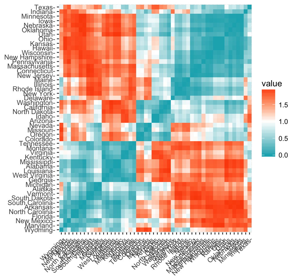
  1. If you use ade4 and FactoMineR (the most used R packages for factor analyses) and you want to make easily a beautiful ggplot2 visualization: then use factoextra, it’s flexible, it has methods for these packages and more.
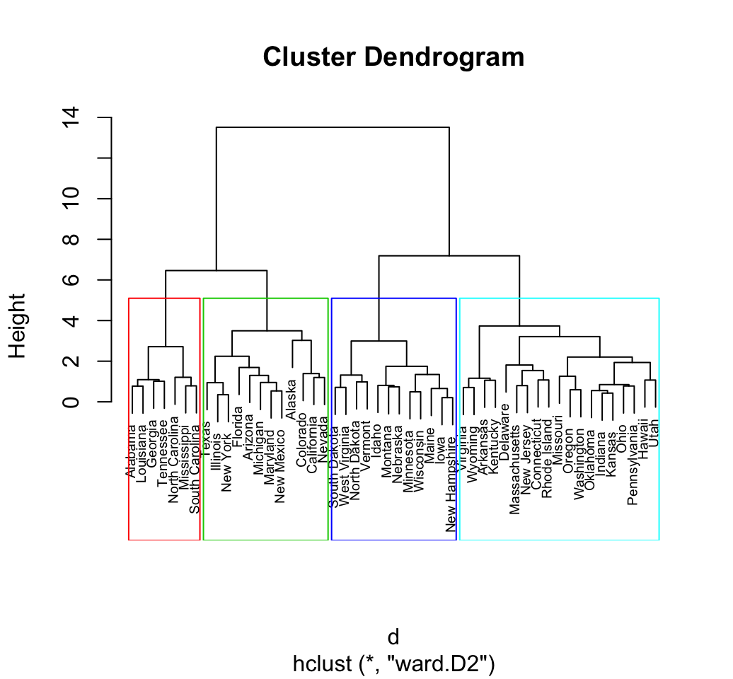
  2. Several functions from different packages are available in R for performing PCA, CA or MCA. However, The components of the output vary from package to package.

No matter the used packages, factoextra can give you a human understandable output.

How to install and load factoextra?

  • factoextra can be installed from CRAN as follow:
install.packages("factoextra")
  • Or, install the latest version from Github
# Install
if(!require(devtools)) install.packages("devtools")
devtools::install_github("kassambara/factoextra")
  • Load factoextra as follow :
library("factoextra")

Main functions in factoextra package

See the online documentation (http://www.sthda.com/english/rpkgs/factoextra) for a complete list. To read more about a given function, click on the corresponding link in the tables below.

Visualizing the outputs of dimension reduction analyses

FunctionsDescription
fviz_eig (or fviz_eigenvalue)Extract and visualize the eigenvalues/variances of dimensions.
fviz_pcaGraph of individuals/variables from the output of Principal Component Analysis (PCA).
fviz_caGraph of column/row variables from the output of Correspondence Analysis (CA).
fviz_mca)Graph of individuals/variables from the output of Multiple Correspondence Analysis (MCA).
fviz_mfaGraph of individuals/variables from the output of Multiple Factor Analysis (MFA).
fviz_hmfaGraph of individuals/variables from the output of Hierarchical Multiple Factor Analysis (HMFA).
fviz_cos2Visualize the quality of the representation of the row/column variable from the results of PCA, CA, MCA functions.
fviz_contribVisualize the contributions of row/column elements from the results of PCA, CA, MCA functions.

Extracting data from the outputs of dimension reduction analyses

FunctionsDescription
get_eigenvalueExtract and visualize the eigenvalues/variances of dimensions.
get_pcaExtract all the results (coordinates, squared cosine, contributions) for the active individuals/variables from Principal Component Analysis (PCA) outputs.
get_caExtract all the results (coordinates, squared cosine, contributions) for the active column/row variables from Correspondence Analysis outputs.
get_mcaExtract results from Multiple Correspondence Analysis outputs.
get_mfaExtract results from Multiple Factor Analysis outputs.
get_hmfaExtract results from Hierarchical Multiple Factor Analysis outputs.
facto_summarizeSubset and summarize the output of factor analyses.

Enhanced clustering analysis and visualization

FunctionsDescription
dist(fviz_dist, get_dist)Enhanced Distance Matrix Computation and Visualization.
get_clust_tendencyAssessing Clustering Tendency.
fviz_nbclust(fviz_gap_stat)Determining and Visualizing the Optimal Number of Clusters.
fviz_dendEnhanced Visualization of Dendrogram
fviz_clusterVisualize Clustering Results
fviz_silhouetteVisualize Silhouette Information from Clustering.
hcutComputes Hierarchical Clustering and Cut the Tree
hkmeans (hkmeans_tree, print.hkmeans)Hierarchical k-means clustering.
eclustVisual enhancement of clustering analysis

Read more about clustering here: Cluster Analysis in R - Unsupervised Machine Learning.

Dimension reduction and factoextra

dimension reduction and factoextra

Principal component analysis

  • Data: iris [Built-in R base dataset]
  • Computing with FactoMineR::PCA()
  • Visualize with factoextra::fviz_pca()

If you want to learn more about computing and interpreting principal component analysis, read this tutorial: Principal Component Analysis (PCA). Here, we provide only a quick start guide.

  1. Loading data
data(iris)
head(iris)
##   Sepal.Length Sepal.Width Petal.Length Petal.Width Species
## 1          5.1         3.5          1.4         0.2  setosa
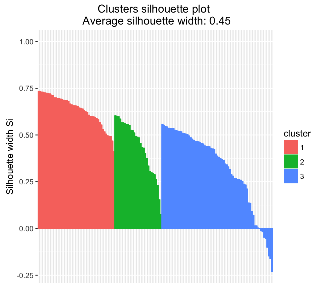
## 2          4.9         3.0          1.4         0.2  setosa
## 3          4.7         3.2          1.3         0.2  setosa
## 4          4.6         3.1          1.5         0.2  setosa
## 5          5.0         3.6          1.4         0.2  setosa
## 6          5.4         3.9          1.7         0.4  setosa
  1. Principal component analysis
# The variable Species (index = 5) is removed before PCA
library("FactoMineR")
res.pca <- PCA(iris[, -5],  graph = FALSE)
  1. Extract and visualize eigenvalues/variances:
# Extract eigenvalues/variances
get_eig(res.pca)
##       eigenvalue variance.percent cumulative.variance.percent
## Dim.1 2.91849782       72.9624454                    72.96245
## Dim.2 0.91403047       22.8507618                    95.81321
## Dim.3 0.14675688        3.6689219                    99.48213
## Dim.4 0.02071484        0.5178709                   100.00000
# Visualize eigenvalues/variances
fviz_eig(res.pca, addlabels=TRUE, hjust = -0.3)+
  theme_minimal()

4.Extract and visualize results for variables:

# Extract the results for variables
var <- get_pca_var(res.pca)
var
## Principal Component Analysis Results for variables
##  ===================================================
##   Name       Description                                    
## 1 "$coord"   "Coordinates for the variables"                
## 2 "$cor"     "Correlations between variables and dimensions"
## 3 "$cos2"    "Cos2 for the variables"                       
## 4 "$contrib" "contributions of the variables"
# Coordinates of variables
head(var$coord)
##                   Dim.1      Dim.2       Dim.3       Dim.4
## Sepal.Length  0.8901688 0.36082989 -0.27565767 -0.03760602
## Sepal.Width  -0.4601427 0.88271627  0.09361987  0.01777631
## Petal.Length  0.9915552 0.02341519  0.05444699  0.11534978
## Petal.Width   0.9649790 0.06399985  0.24298265 -0.07535950
# Contribution of variables
head(var$contrib)
##                  Dim.1       Dim.2     Dim.3     Dim.4
## Sepal.Length 27.150969 14.24440565 51.777574  6.827052
## Sepal.Width   7.254804 85.24748749  5.972245  1.525463
## Petal.Length 33.687936  0.05998389  2.019990 64.232089
## Petal.Width  31.906291  0.44812296 40.230191 27.415396
# Graph of variables: default plot
fviz_pca_var(res.pca, col.var = "steelblue")

It’s possible to control variable colors using their contributions to the principal axes:

# Control variable colors using their contributions
# Use gradient color
fviz_pca_var(res.pca, col.var="contrib")+
scale_color_gradient2(low="white", mid="blue", 
      high="red", midpoint = 96) +
theme_minimal()

  1. Variable contributions to the principal axes:
# Variable contributions on axis 1
fviz_contrib(res.pca, choice="var", axes = 1 )+
  labs(title = "Contributions to Dim 1")

# Variable contributions on axes 1 + 2
fviz_contrib(res.pca, choice="var", axes = 1:2)+
  labs(title = "Contributions to Dim 1+2")

  1. Extract and visualize results for individuals:
# Extract the results for individuals
ind <- get_pca_ind(res.pca)
ind
## Principal Component Analysis Results for individuals
##  ===================================================
##   Name       Description                       
## 1 "$coord"   "Coordinates for the individuals" 
## 2 "$cos2"    "Cos2 for the individuals"        
## 3 "$contrib" "contributions of the individuals"
# Coordinates of individuals
head(ind$coord)
##       Dim.1      Dim.2       Dim.3       Dim.4
## 1 -2.264703  0.4800266 -0.12770602 -0.02416820
## 2 -2.080961 -0.6741336 -0.23460885 -0.10300677
## 3 -2.364229 -0.3419080  0.04420148 -0.02837705
## 4 -2.299384 -0.5973945  0.09129011  0.06595556
## 5 -2.389842  0.6468354  0.01573820  0.03592281
## 6 -2.075631  1.4891775  0.02696829 -0.00660818
# Graph of individuals
# 1. Use repel = TRUE to avoid overplotting
# 2. Control automatically the color of individuals using the cos2
    # cos2 = the quality of the individuals on the factor map
    # Use points only
# 3. Use gradient color
fviz_pca_ind(res.pca, repel = TRUE, col.ind = "cos2")+
  scale_color_gradient2(low="blue", mid="white",
      high="red", midpoint=0.6)+
  theme_minimal()

# Color by groups: habillage=iris$Species
# Show points only: geom = "point"
p <- fviz_pca_ind(res.pca, geom = "point",
    habillage=iris$Species, addEllipses=TRUE,
    ellipse.level= 0.95)+ theme_minimal()
print(p)

# Change group colors manually
# Read more: http://www.sthda.com/english/wiki/ggplot2-colors
p + scale_color_manual(values=c("#999999", "#E69F00", "#56B4E9"))+
 scale_fill_manual(values=c("#999999", "#E69F00", "#56B4E9"))+
 theme_minimal()    

# Biplot of individuals and variables
# ++++++++++++++++++++++++++
# Only variables are labelled
 fviz_pca_biplot(res.pca,  label="var", habillage=iris$Species,
      addEllipses=TRUE, ellipse.level=0.95) +
  theme_minimal()

Correspondence analysis

  • Data: housetasks [in factoextra]
  • Computing with FactoMineR::CA()
  • Visualize with factoextra::fviz_ca()

If you want to learn more about computing and interpreting correspondence analysis, read this tutorial: Correspondence Analysis (CA). Here, we provide only a quick start guide.

 # 1. Loading data
data("housetasks")
head(housetasks)
##            Wife Alternating Husband Jointly
## Laundry     156          14       2       4
## Main_meal   124          20       5       4
## Dinner       77          11       7      13
## Breakfeast   82          36      15       7
## Tidying      53          11       1      57
## Dishes       32          24       4      53
 # 2. Computing CA
library("FactoMineR")
res.ca <- CA(housetasks, graph = FALSE)

# 3. Extract results for row/column variables
# ++++++++++++++++++++++++++++++++
# Result for row variables
get_ca_row(res.ca)
## Correspondence Analysis - Results for rows
##  ===================================================
##   Name       Description                
## 1 "$coord"   "Coordinates for the rows" 
## 2 "$cos2"    "Cos2 for the rows"        
## 3 "$contrib" "contributions of the rows"
## 4 "$inertia" "Inertia of the rows"
# Result for column variables
get_ca_col(res.ca)
## Correspondence Analysis - Results for columns
##  ===================================================
##   Name       Description                   
## 1 "$coord"   "Coordinates for the columns" 
## 2 "$cos2"    "Cos2 for the columns"        
## 3 "$contrib" "contributions of the columns"
## 4 "$inertia" "Inertia of the columns"
# 4. Visualize row/column variables
# ++++++++++++++++++++++++++++++++
# Visualize row contributions on axes 1
fviz_contrib(res.ca, choice ="row", axes = 1)

# Visualize column contributions on axes 1
fviz_contrib(res.ca, choice ="col", axes = 1)

# 5. Graph of row variables
fviz_ca_row(res.ca, repel = TRUE)

# Graph of column points
fviz_ca_col(res.ca)

# Biplot of rows and columns
fviz_ca_biplot(res.ca, repel = TRUE)

Multiple correspondence analysis

  • Data: poison [in factoextra]
  • Computing with FactoMineR::MCA()
  • Visualize with factoextra::fviz_mca()

If you want to learn more about computing and interpreting multiple correspondence analysis, read this tutorial: Multiple Correspondence Analysis (MCA). Here, we provide only a quick start guide.

  1. Computing MCA:
library(FactoMineR)
data(poison)
res.mca <- MCA(poison, quanti.sup = 1:2,
              quali.sup = 3:4, graph=FALSE)
  1. Extract results for variables and individuals:
# Extract the results for variable categories
get_mca_var(res.mca)

# Extract the results for individuals
get_mca_ind(res.mca)
  1. Contribution of variables and individuals to the principal axes:
# Visualize variable categorie contributions on axes 1
fviz_contrib(res.mca, choice ="var", axes = 1)

# Visualize individual contributions on axes 1
# select the top 20
fviz_contrib(res.mca, choice ="ind", axes = 1, top = 20)
  1. Graph of individuals
# Color by groups
# Add concentration ellipses
# Use repel = TRUE to avoid overplotting
grp <- as.factor(poison[, "Vomiting"])
fviz_mca_ind(res.mca, col.ind = "blue", habillage = grp,
             addEllipses = TRUE, repel = TRUE)+
   theme_minimal()

  1. Graph of variable categories:
fviz_mca_var(res.mca, repel = TRUE)

It’s possible to select only some variables:

# Select the top 10 contributing variable categories
fviz_mca_var(res.mca, select.var = list(contrib = 10))
# Select by names
fviz_mca_var(res.mca,
 select.var= list(name = c("Courg_n", "Fever_y", "Fever_n")))
  1. Biplot of individuals and variables:
fviz_mca_biplot(res.mca, repel = TRUE)+
  theme_minimal()

# Select the top 30 contributing individuals
# And the top 10 variables
fviz_mca_biplot(res.mca,
               select.ind = list(contrib = 30),
               select.var = list(contrib = 10))

Multiple factor analysis

  • Data: wine [in factoextra]
  • Computing with FactoMineR::MFA()
  • Visualize with factoextra::fviz_mfa()

If you want to learn more about computing and interpreting multiple factor analysis, read this tutorial: Multiple Factor Analysis (MCA). Here, we provide only a quick start guide.

  1. Computing MFA:
library(FactoMineR)
data(wine)
res.mfa <- MFA(wine, group=c(2,5,3,10,9,2), type=c("n",rep("s",5)),
               ncp=5, name.group=c("orig","olf","vis","olfag","gust","ens"),
               num.group.sup=c(1,6), graph=FALSE)
  1. Graph of individuals:
fviz_mfa_ind(res.mfa)
# Graph of partial individuals (starplot)
fviz_mfa_ind_starplot(res.mfa, col.partial = "group.name",
                      repel = TRUE)+
  scale_color_brewer(palette = "Dark2")+
  theme_minimal()

  1. Graph of quantitative variables:
fviz_mfa_quanti_var(res.mfa)

Cluster analysis and factoextra

Partitioning clustering

Partitioning cluster analysis

# 1. Loading and preparing data
data("USArrests")
df <- scale(USArrests)

# 2. Compute k-means
set.seed(123)
km.res <- kmeans(scale(USArrests), 4, nstart = 25)

# 3. Visualize
library("factoextra")
fviz_cluster(km.res, data = df)+theme_minimal()+
  scale_color_manual(values = c("#00AFBB","#2E9FDF", "#E7B800", "#FC4E07"))+
  scale_fill_manual(values = c("#00AFBB","#2E9FDF", "#E7B800", "#FC4E07")) +
  labs(title= "Partitioning Clustering Plot")


Hierarchical clustering

Hierarchical clustering

library("factoextra")
# Compute hierarchical clustering and cut into 4 clusters
res <- hcut(USArrests, k = 4, stand = TRUE)

# Visualize
fviz_dend(res, rect = TRUE, cex = 0.5,
          k_colors = c("#00AFBB","#2E9FDF", "#E7B800", "#FC4E07"))


Determine the optimal number of clusters

# Optimal number of clusters for k-means
library("factoextra")
my_data <- scale(USArrests)
fviz_nbclust(my_data, kmeans, method = "gap_stat")


Infos

This analysis has been performed using R software (ver. 3.2.4) and factoextra (ver. 1.0.3)

Computing and Adding new Variables to a Data Frame in R

$
0
0


Previously, we described the essentials of R programming and provided quick start guides for importing data into R as well as converting your data into a tibble data format, which is modern convention way to work with your data. We also described crutial steps to reshape your data with R for easier analyses.


Here, you we’ll learn how to compute and add new variables to a data frame in R. This can be done easily using the functions mutate() and transmute() in dplyr R package.


  • mutate(): Computes and adds new variable(s). Preserves existing variables. It’s similar to the R base function transform().
  • transmute(): Computes new variable(s). Drops existing variables.

Renaming Columns of a Data Table in R
Figure adapted from RStudio data wrangling cheatsheet

Pleleminary tasks

  1. Launch RStudio as described here: Running RStudio and setting up your working directory

  2. Prepare your data as described here: Best practices for preparing your data and save it in an external .txt tab or .csv files

  3. Import your data into R as described here: Fast reading of data from txt|csv files into R: readr package.

Here, we’ll use the R built-in iris data set, which we start by converting to a tibble data frame (tbl_df). Tibble is a modern rethinking of data frame providing a nicer printing method. This is useful when working with large data sets.

# Create my_data
my_data <- iris[, -5]

# Convert to a tibble
library("tibble")
my_data <- as_data_frame(my_data)

# Print
my_data
Source: local data frame [150 x 4]

   Sepal.Length Sepal.Width Petal.Length Petal.Width
          <dbl>       <dbl>        <dbl>       <dbl>
1           5.1         3.5          1.4         0.2
2           4.9         3.0          1.4         0.2
3           4.7         3.2          1.3         0.2
4           4.6         3.1          1.5         0.2
5           5.0         3.6          1.4         0.2
6           5.4         3.9          1.7         0.4
7           4.6         3.4          1.4         0.3
8           5.0         3.4          1.5         0.2
9           4.4         2.9          1.4         0.2
10          4.9         3.1          1.5         0.1
..          ...         ...          ...         ...

Install and load dplyr package for renaming columns

  • Install dplyr
install.packages("dplyr")
  • Load dplyr:
library("dplyr")

dplyr::mutate(): Add new variables by preserving existing ones

  • Add new columns (sepal_by_petal_*) by preserving existing ones:
mutate(my_data,
       sepal_by_petal_l = Sepal.Length/Petal.Length
       )
Source: local data frame [150 x 5]

   Sepal.Length Sepal.Width Petal.Length Petal.Width sepal_by_petal_l
          (dbl)       (dbl)        (dbl)       (dbl)            (dbl)
1           5.1         3.5          1.4         0.2         3.642857
2           4.9         3.0          1.4         0.2         3.500000
3           4.7         3.2          1.3         0.2         3.615385
4           4.6         3.1          1.5         0.2         3.066667
5           5.0         3.6          1.4         0.2         3.571429
6           5.4         3.9          1.7         0.4         3.176471
7           4.6         3.4          1.4         0.3         3.285714
8           5.0         3.4          1.5         0.2         3.333333
9           4.4         2.9          1.4         0.2         3.142857
10          4.9         3.1          1.5         0.1         3.266667
..          ...         ...          ...         ...              ...

dplyr::transmute(): Make new variables by dropping existing ones

  • Add new columns (sepal_by_petal_*) by dropping existing ones:
transmute(my_data, 
            sepal_by_petal_l = Sepal.Length/Petal.Length,
            sepal_by_petal_w = Sepal.Width/Petal.Width
            )
Source: local data frame [150 x 2]

   sepal_by_petal_l sepal_by_petal_w
              (dbl)            (dbl)
1          3.642857         17.50000
2          3.500000         15.00000
3          3.615385         16.00000
4          3.066667         15.50000
5          3.571429         18.00000
6          3.176471          9.75000
7          3.285714         11.33333
8          3.333333         17.00000
9          3.142857         14.50000
10         3.266667         31.00000
..              ...              ...

Use mutate() and transmute() programmatically inside a function:


mutate() and transmute() are best-suited for interactive use. The functions mutate_() and transmute() should be used for calling from a function. In this case the input must be “quoted”.


There are three ways to quote inputs that dplyr understands:

  • With a formula, ~Sepal.Length.
  • With quote(), quote(Sepal.Length).
  • As a string: “Sepal.Length”.
# Use formula
mutate_(my_data, 
            sepal_by_petal_l = ~Sepal.Length/Petal.Length,
            sepal_by_petal_w = ~Sepal.Width/Petal.Width
            )

# Or use quote
transmute_(my_data, 
            sepal_by_petal_l = quote(Sepal.Length/Petal.Length),
            sepal_by_petal_w = quote(Sepal.Width/Petal.Width)
            )

# or, this
transmute_(my_data, 
            sepal_by_petal_l = "Sepal.Length/Petal.Length",
            sepal_by_petal_w = "Sepal.Width/Petal.Width"
            )

transform(): R base function to compute and add new variables

dplyr::mutate() works similarly to the R base function transform(), except that in mutate() you can refer to variables you’ve just created. This is not possible in transform().

my_data2 <- transform(my_data, neg_sepal_length = -Sepal.Length)
head(my_data2)
  Sepal.Length Sepal.Width Petal.Length Petal.Width neg_sepal_length
1          5.1         3.5          1.4         0.2             -5.1
2          4.9         3.0          1.4         0.2             -4.9
3          4.7         3.2          1.3         0.2             -4.7
4          4.6         3.1          1.5         0.2             -4.6
5          5.0         3.6          1.4         0.2             -5.0
6          5.4         3.9          1.7         0.4             -5.4

Summary


  • dplyr::mutate(iris, sepal = 2*Sepal.Length): Computes and appends new variable(s).
  • dplyr::transmute(iris, sepal = 2*Sepal.Length): Makes new variable(s) and drops existing ones.
  • transform(iris, sepal = 2*Sepal.Length): R base function similar to mutate().


Infos

This analysis has been performed using R (ver. 3.2.4).

Line Plots - R Base Graphs

$
0
0


Previously, we described the essentials of R programming and provided quick start guides for importing data into R.


Here, we’ll describe how to create line plots in R. The function plot() or lines() can be used to create a line plot.


Pleleminary tasks

  1. Launch RStudio as described here: Running RStudio and setting up your working directory

  2. Prepare your data as described here: Best practices for preparing your data and save it in an external .txt tab or .csv files

  3. Import your data into R as described here: Fast reading of data from txt|csv files into R: readr package.

R base functions: plot() and lines()

The simplified format of plot() and lines() is as follow.

plot(x, y, type = "l", lty = 1)

lines(x, y, type = "l", lty = 1)

  • x, y: coordinate vectors of points to join
  • type: character indicating the type of plotting. Allowed values are:
    • “p” for points
    • “l” for lines
    • “b” for both points and lines
    • “c” for empty points joined by lines
    • “o” for overplotted points and lines
    • “s” and “S” for stair steps
    • “n” does not produce any points or lines
  • lty: line types. Line types can either be specified as an integer (0=blank, 1=solid (default), 2=dashed, 3=dotted, 4=dotdash, 5=longdash, 6=twodash) or as one of the character strings “blank”, “solid”, “dashed”, “dotted”, “dotdash”, “longdash”, or “twodash”, where “blank” uses ‘invisible lines’ (i.e., does not draw them).


Create some data

# Create some variables
x <- 1:10
y1 <- x*x
y2  <- 2*y1

We’ll plot a plot with two lines: lines(x, y1) and lines(x, y2).

Note that the function lines() can not produce a plot on its own. However, it can be used to add lines() on an existing graph. This means that, first you have to use the function plot() to create an empty graph and then use the function lines() to add lines.

Basic line plots

# Create a basic stair steps plot 
plot(x, y1, type = "S")

# Show both points and line
plot(x, y1, type = "b", pch = 19, 
     col = "red", xlab = "x", ylab = "y")

Plots with multiple lines

# Create a first line
plot(x, y1, type = "b", frame = FALSE, pch = 19, 
     col = "red", xlab = "x", ylab = "y")

# Add a second line
lines(x, y2, pch = 18, col = "blue", type = "b", lty = 2)

# Add a legend to the plot
legend("topleft", legend=c("Line 1", "Line 2"),
       col=c("red", "blue"), lty = 1:2, cex=0.8)

Infos

This analysis has been performed using R statistical software (ver. 3.2.4).

Pie Charts - R Base Graphs

$
0
0


Previously, we described the essentials of R programming and provided quick start guides for importing data into R.


Here, we’ll describe how to create pie charts in R. The R base function pie() can be used for this.


Pleleminary tasks

  1. Launch RStudio as described here: Running RStudio and setting up your working directory

  2. Prepare your data as described here: Best practices for preparing your data and save it in an external .txt tab or .csv files

  3. Import your data into R as described here: Fast reading of data from txt|csv files into R: readr package.

Create some data

df <- data.frame(
  group = c("Male", "Female", "Child"),
  value = c(25, 25, 50)
  )

df
##    group value
## 1   Male    25
## 2 Female    25
## 3  Child    50

Create basic pie charts: pie()

The function pie() can be used to draw a pie chart.

pie(x, labels = names(x), radius = 0.8)

  • x: a vector of non-negative numerical quantities. The values in x are displayed as the areas of pie slices.
  • labels: character strings giving names for the slices.
  • radius: radius of the pie circle. If the character strings labeling the slices are long it may be necessary to use a smaller radius.


pie(df$value, labels = df$group, radius = 1)

# Change colors
pie(df$value, labels = df$group, radius = 1,
    col = c("#999999", "#E69F00", "#56B4E9"))

Create 3D pie charts: plotix::pie3D()

Te function pie3D()[in plotrix package] can be used to draw a 3D pie chart.

Install plotrix package:

install.packages("plotrix")

Use pie3D():

# 3D pie chart
library("plotrix")
pie3D(df$value, labels = df$group, radius = 1.5, 
      col = c("#999999", "#E69F00", "#56B4E9"))

# Explode the pie chart
pie3D(df$value, labels = df$group, radius = 1.5,
      col = c("#999999", "#E69F00", "#56B4E9"),
      explode = 0.1)

Infos

This analysis has been performed using R statistical software (ver. 3.2.4).

Viewing all 183 articles
Browse latest View live