- 1 Required package
- 2 K-means clustering
- 3 PAM: Partitioning Around Medoids
- 4 CLARA: Clustering Large Applications
- 5 R packages and functions for visualizing partitioning clusters
- 6 Infos
Clustering is a data exploratory technique used for discovering groups or pattern in a dataset. There are two standard clustering strategies: partitioning methods and hierarchical clustering.
This article describes the most well-known and commonly used partitioning algorithms including:
- K-means clustering (MacQueen, 1967), in which, each cluster is represented by the center or means of the data points belonging to the cluster.
- K-medoids clustering or PAM (Partitioning Around Medoids, Kaufman & Rousseeuw, 1990), in which, each cluster is represented by one of the objects in the cluster. Well describe also a variant of PAM named CLARA (Clustering Large Applications) which is used for analyzing large data sets.
For each of these methods, we provide:
- the basic idea and the key mathematical concepts
- the clustering algorithm and implementation in R software
- R lab sections with many examples for computing clustering methods and visualizing the outputs
1 Required package
The only required packages for this chapter are:
- cluster for computing PAM and CLARA
- factoextra which will be used to visualize clusters.
- Install factoextra package as follow:
if(!require(devtools)) install.packages("devtools")
devtools::install_github("kassambara/factoextra")- Install cluster package as follow:
install.packages("cluster")- Load the packages :
library(cluster)
library(factoextra)
2 K-means clustering
K-means clustering is the simplest and the most commonly used partitioning method for splitting a dataset into a set of k groups (i.e. clusters). It requires the analyst to specify the number of optimal clusters to be generated from the data.
2.1 Concept
Generally, clustering is defined as grouping objects in sets, such that objects within a cluster are as similar as possible, whereas objects from different clusters are as dissimilar as possible. A good clustering will generate clusters with a high intra-class similarity and a low inter-class similarity.
Hence, the basic idea behind K-means clustering consists of defining clusters so that the total intra-cluster variation (known as total within-cluster variation) is minimized.
The equation to be solved can be defined as follow:
\(minimize\left(\sum\limits_{k=1}^k W(C_k)\right)\),
Where \(C_k\) is the \(k_{th}\) cluster and \(W(C_k)\) is the within-cluster variation of the cluster \(C_k\).
What is the formula of \(W(C_k)\)?
There are many ways to define the within-cluster variation (\(W(C_k)\)). The algorithm of Hartigan and Wong (1979) is used by default in R software. It uses Euclidean distance measures between data points to determine the within- and the between-cluster similarities.
Each observation is assigned to a given cluster such that the sum of squares (SS) of the observation to their assigned cluster centers is a minimum.
To solve the equation presented above, the within-cluster variation (\(W(C_k)\)) for a given cluster \(C_k\), containing \(n_k\) points, can be defined as follow:

\[ W(C_k) = \frac{1}{n_k}\sum\limits_{x_i \in C_k}\sum\limits_{x_j \in C_k} (x_i - x_j)^2 = \sum\limits_{x_i \in C_k} (x_i - \mu_k)^2 \]
- \(x_i\) design a data point belonging to the cluster \(C_k\)
- \(\mu_k\) is the mean value of the points assigned to the cluster \(C_k\)
The within-cluster variation for a cluster \(C_k\) with \(n_k\) number of points is the sum of all of the pairwise squared Euclidean distances between the observations \(C_k\), divided by \(n_k\).
We define the total within-cluster sum of square (i.e, total within-cluster variation) as follow:
\[ tot.withinss = \sum\limits_{k=1}^k W(C_k) = \sum\limits_{k=1}^k \sum\limits_{x_i \in C_k} (x_i - \mu_k)^2 \]
The total within-cluster sum of square measures the compactness (i.e goodness) of the clustering and we want it to be as small as possible.
2.2 Algorithm
In k-means clustering, each cluster is represented by its center (i.e, centroid) which corresponds to the mean of points assigned to the cluster. Recall that, k-means algrorithm requires the user to choose the number of clusters (i.e, k) to be generated.
The algorithm starts by randomly selecting k objects from the dataset as the initial cluster means.
Next, each of the remaining objects is assigned to its closest centroid, where closest is defined using the Euclidean distance between the object and the cluster mean. This step is called cluster assignement step.
After the assignment step, the algorithm computes the new mean value of each cluster. The term cluster centroid update is used to design this step. All the objects are reassigned again using the updated cluster means.
The cluster assignment and centroid update steps are iteratively repeated until the cluster assignments stop changing (i.e until convergence is achieved). That is, the clusters formed in the current iteration are the same as those obtained in the previous iteration.
The algorithm can be summarize as follow:
- Specify the number of clusters (K) to be created (by the analyst)
- Select randomly k objects from the dataset as the initial cluster centers or means
- Assigns each observation to their closest centroid, based on the Euclidean distance between the object and the centroid
- For each of the k clusters update the cluster centroid by calculating the new mean values of all the data points in the cluster. The centoid of a \(K_{th}\) cluster is a vector of length p containing the means of all variables for the observations in the \(k_{th}\) cluster; p is the number of variables.
- Iteratively minimize the total within sum of square. That is, iterate steps 3 and 4 until the cluster assignments stop changing or the maximum number of iterations is reached. By default R uses 10 as the default value for the maximum number of iterations.
Note that, k-means clustering is very simple and efficient algorithm. However there are some weaknesses, including:
- It assumes prior knowledge of the data and requires the analyst to choose the appropriate k in advance
- The final results obtained is sensitive to the initial random selection of cluster centers.
How to overcome these 2 difficulties?
Well describe the solutions to each of these two disadvantages in the next sections. Briefly the solutions are:
- Solution to issue 1: Compute k-means for a range of k values, for example by varying k between 2 and 20. Then, choose the best k by comparing the clustering results obtained for the different k values. This will be described comprehensively in the chapter named: cluster evaluation and validation statistics
- Solution to issue 2: K-means algorithm is computed several times with different initial cluster centers. The run with the lowest total within-cluster sum of square is selected as the final clustering solution. This is described in the following section.
2.3 R function for k-means clustering
K-mean clustering must be performed only on a data in which all variables are continuous as the algorithm uses variable means.
The standard R function for k-means clustering is kmeans() [in stats package]. A simplified format is:
kmeans(x, centers, iter.max = 10, nstart = 1)- x: numeric matrix, numeric data frame or a numeric vector
- centers: Possible values are the number of clusters (k) or a set of initial (distinct) cluster centers. If a number, a random set of (distinct) rows in x is chosen as the initial centers.
- iter.max: The maximum number of iterations allowed. Default value is 10.
- nstart: The number of random starting partitions when centers is a number. Trying nstart > 1 is often recommended.
kmeans() function returns a list including:
- cluster: A vector of integers (from 1:k) indicating the cluster to which each point is allocated
- centers: A matrix of cluster centers (cluster means)
- totss: The total sum of squares (TSS), i.e \(\sum{(x_i - \bar{x})^2}\). TSS measures the total variance in the data.
- withinss: Vector of within-cluster sum of squares, one component per cluster
- tot.withinss: Total within-cluster sum of squares, i.e. \(sum(withinss)\)
- betweenss: The between-cluster sum of squares, i.e. \(totss - tot.withinss\)
- size: The number of observations in each cluster
As k-means clustering algorithm starts with k randomly selected centroids, its always recommended to use the set.seed() function in order to set a seed for Rs random number generator.
The aim is to make reproducible the results, so that the reader of this article will obtain exactly the same results as those shown below.2.4 Data format
The R code below generates a two-dimensional simulated data format which will be used for performing k-means clustering:
set.seed(123)
# Two-dimensional data format
df <- rbind(matrix(rnorm(100, sd = 0.3), ncol = 2),
           matrix(rnorm(100, mean = 1, sd = 0.3), ncol = 2))
colnames(df) <- c("x", "y")
head(df)
## x y
## [1,] -0.16814269 0.075995554
## [2,] -0.06905325 -0.008564027
## [3,] 0.46761249 -0.012861137
## [4,] 0.02115252 0.410580685
## [5,] 0.03878632 -0.067731296
## [6,] 0.51451950 0.4549411812.5 Compute k-means clustering
The R code below performs k-means clustering with k = 2:
# Compute k-means
set.seed(123)
km.res <- kmeans(df, 2, nstart = 25)
# Cluster number for each of the observations
km.res$cluster
## [1] 1 1 1 1 1 1 1 1 1 1 1 1 1 1 1 1 1 1 1 1 1 1 1 1 1 1 1 1 1 1 1 1 1 1 1
## [36] 1 1 1 1 1 1 1 1 1 1 1 1 1 1 1 2 2 2 2 2 2 2 2 2 2 2 2 2 2 2 2 2 2 2 2
## [71] 2 2 2 2 2 2 2 2 2 2 2 2 2 2 2 2 2 2 2 2 2 2 2 2 2 2 2 2 2 2# Cluster size
km.res$size## [1] 50 50# Cluster means
km.res$centers## x y
## 1 0.01032106 0.04392248
## 2 0.92382987 1.01164205Its possible to plot the data with coloring each data point according to its cluster assignment. The cluster centers are specified using big stars:
plot(df, col = km.res$cluster, pch = 19, frame = FALSE,
     main = "K-means with k = 2")
points(km.res$centers, col = 1:2, pch = 8, cex = 3)
OK, cool! The data points are perfectly partitioned!! But why didnt you perform k-means clustering with k = 3 or 4 rather than using k = 2?
The data used in the example above is a simulated data and we knew exactly that there are only 2 real clusters.
For real data, we could have tried the clustering with k = 3 or 4. Lets try it with k = 4 as follow:
set.seed(123)
km.res <- kmeans(df, 4, nstart = 25)
plot(df, col = km.res$cluster, pch = 19, frame = FALSE,
     main = "K-means with k = 4")
points(km.res$centers, col = 1:4, pch = 8, cex = 3)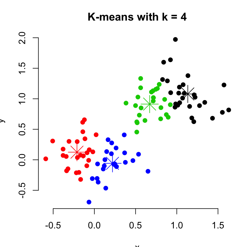
# Print the result
km.res
## K-means clustering with 4 clusters of sizes 27, 25, 24, 24
##
## Cluster means:
## x y
## 1 1.1336807 1.07876045
## 2 -0.2110757 0.12500530
## 3 0.6706931 0.91293798
## 4 0.2199345 -0.05766457
##
## Clustering vector:
## [1] 2 2 4 2 4 3 4 2 2 2 4 4 4 4 2 4 4 2 4 2 2 4 2 2 2 2 4 4 2 4 4 2 4 4 4
## [36] 4 4 2 2 2 2 2 2 4 4 2 2 2 4 4 3 1 1 3 3 1 3 3 1 1 1 1 3 1 1 1 1 3 3 3
## [71] 1 3 3 1 1 3 1 1 3 1 1 1 1 3 3 1 3 1 1 3 1 3 3 3 3 1 3 1 1 3
##
## Within cluster sum of squares by cluster:
## [1] 3.786069 2.096232 1.747682 2.184534
## (between_SS / total_SS = 83.6 %)
##
## Available components:
##
## [1] "cluster" "centers" "totss" "withinss"
## [5] "tot.withinss" "betweenss" "size" "iter"
## [9] "ifault"A method, for estimating the optimal number of clusters in the data, is presented in the next section.
What means nstart? Why did you use the argument nstart = 25 rather than nstart = 1?
Excellent question! As mentioned in the previous sections, one disadvantage of k-means clustering is the sensitivity of the final results to the initial random centroids.
The option nstart is the number of random sets to be chosen at Step 2 of the k-means algorithm. The default value of nstart in R is one. But, Its recommended to try more than one random start (i.e. use nstart > 1).
In other words, if the value of nstart is greater than one, then k-means clustering algorithm will start by defining multiple random configurations (Step 2 of the algorithm). For instance, if \(nstart = 50\), the algorithm will create 50 initial configurations. Finally, kmeans() function will report only the best results.
In conclusion, if you want the algorithm to do a good job, try several random starts (nstart > 1).
As mentioned above, a good k-means clustering is a one that minimize the total within-cluster variation (i.e, the average distance of each point to its assigned centroid). For illustration, lets compare the results (i.e. tot.withinss) of a k-means approach with nstart = 1 against nstart = 25.
set.seed(123)
# K-means with nstart = 1
km.res <- kmeans(df, 4, nstart = 1)
km.res$tot.withinss
## [1] 10.13198# K-means with nstart = 25
km.res <- kmeans(df, 4, nstart = 25)
km.res$tot.withinss## [1] 9.814517It can be seen that the tot.withinss is further improved (i.e. minimized) when the value of nstart is large.
Note that, its strongly recommended to compute k-means clustering with a large value of nstart such as 25 or 50, in order to have a more stable result.
2.6 Application of K-means clustering on real data
2.6.1 Data preparation and descriptive statistics
Well use the built-in R dataset USArrest which contains statistics, in arrests per 100,000 residents for assault, murder, and rape in each of the 50 US states in 1973. It includes also the percent of the population living in urban areas.
It contains 50 observations on 4 variables:
- [,1] Murder numeric Murder arrests (per 100,000)
- [,2] Assault numeric Assault arrests (per 100,000)
- [,3] UrbanPop numeric Percent urban population
- [,4] Rape numeric Rape arrests (per 100,000)
# Load the data set
data("USArrests")

# Remove any missing value (i.e, NA values for not available)
# That might be present in the data
df <- na.omit(USArrests)

# View the firt 6 rows of the data
head(df, n = 6)
## Murder Assault UrbanPop Rape
## Alabama 13.2 236 58 21.2
## Alaska 10.0 263 48 44.5
## Arizona 8.1 294 80 31.0
## Arkansas 8.8 190 50 19.5
## California 9.0 276 91 40.6
## Colorado 7.9 204 78 38.7Before k-means clustering, we can compute some descriptive statistics:
desc_stats <- data.frame(
  Min = apply(df, 2, min), # minimum
  Med = apply(df, 2, median), # median
  Mean = apply(df, 2, mean), # mean
  SD = apply(df, 2, sd), # Standard deviation
  Max = apply(df, 2, max) # Maximum
  )
desc_stats <- round(desc_stats, 1)
head(desc_stats)
## Min Med Mean SD Max
## Murder 0.8 7.2 7.8 4.4 17.4
## Assault 45.0 159.0 170.8 83.3 337.0
## UrbanPop 32.0 66.0 65.5 14.5 91.0
## Rape 7.3 20.1 21.2 9.4 46.0Note that the variables have a large different means and variances. This is explained by the fact that the variables are measured in different units; Murder, Rape, and Assault are measured as the number of occurrences per 100 000 people, and UrbanPop is the percentage of the states population that lives in an urban area.
They must be standardized (i.e., scaled) to make them comparable. Recall that, standardization consists of transforming the variables such that they have mean zero and standard deviation one. You can read more about standardization in the following article: distance measures and scaling.
As we dont want the k-means algorithm to depend to an arbitrary variable unit, we start by scaling the data using the R function scale() as follow:
df <- scale(df)
head(df)
## Murder Assault UrbanPop Rape
## Alabama 1.24256408 0.7828393 -0.5209066 -0.003416473
## Alaska 0.50786248 1.1068225 -1.2117642 2.484202941
## Arizona 0.07163341 1.4788032 0.9989801 1.042878388
## Arkansas 0.23234938 0.2308680 -1.0735927 -0.184916602
## California 0.27826823 1.2628144 1.7589234 2.067820292
## Colorado 0.02571456 0.3988593 0.8608085 1.8649672072.6.2 Determine the number of optimal clusters in the data
Partitioning methods require the users to specify the number of clusters to be generated.
One fundamental question is: How to choose the right number of expected clusters (k)?
Different methods will be presented in the chapter cluster evaluation and validation statistics.
Here, we provide a simple solution. The idea is to compute a clustering algorithm of interest using different values of clusters k. Next, the wss (within sum of square) is drawn according to the number of clusters. The location of a bend (knee) in the plot is generally considered as an indicator of the appropriate number of clusters.
Well use the function fviz_nbclust() [in factoextra package] which format is:
fviz_nbclust(x, FUNcluster, method = c("silhouette", "wss"))- x: numeric matrix or data frame
- FUNcluster: a partitioning function such as kmeans, pam, clara etc
- method: the method to be used for determining the optimal number of clusters.
The R code below computes the elbow method for kmeans():
library(factoextra)
set.seed(123)
fviz_nbclust(df, kmeans, method = "wss") +
    geom_vline(xintercept = 4, linetype = 2)
Four clusters are suggested.
2.6.3 Compute k-means clustering
# Compute k-means clustering with k = 4
set.seed(123)
km.res <- kmeans(df, 4, nstart = 25)
print(km.res)
## K-means clustering with 4 clusters of sizes 13, 16, 13, 8
##
## Cluster means:
## Murder Assault UrbanPop Rape
## 1 -0.9615407 -1.1066010 -0.9301069 -0.96676331
## 2 -0.4894375 -0.3826001 0.5758298 -0.26165379
## 3 0.6950701 1.0394414 0.7226370 1.27693964
## 4 1.4118898 0.8743346 -0.8145211 0.01927104
##
## Clustering vector:
## Alabama Alaska Arizona Arkansas California
## 4 3 3 4 3
## Colorado Connecticut Delaware Florida Georgia
## 3 2 2 3 4
## Hawaii Idaho Illinois Indiana Iowa
## 2 1 3 2 1
## Kansas Kentucky Louisiana Maine Maryland
## 2 1 4 1 3
## Massachusetts Michigan Minnesota Mississippi Missouri
## 2 3 1 4 3
## Montana Nebraska Nevada New Hampshire New Jersey
## 1 1 3 1 2
## New Mexico New York North Carolina North Dakota Ohio
## 3 3 4 1 2
## Oklahoma Oregon Pennsylvania Rhode Island South Carolina
## 2 2 2 2 4
## South Dakota Tennessee Texas Utah Vermont
## 1 4 3 2 1
## Virginia Washington West Virginia Wisconsin Wyoming
## 2 2 1 1 2
##
## Within cluster sum of squares by cluster:
## [1] 11.952463 16.212213 19.922437 8.316061
## (between_SS / total_SS = 71.2 %)
##
## Available components:
##
## [1] "cluster" "centers" "totss" "withinss"
## [5] "tot.withinss" "betweenss" "size" "iter"
## [9] "ifault"Its possible to compute the mean of each of the variables in the clusters:
aggregate(USArrests, by=list(cluster=km.res$cluster), mean)## cluster Murder Assault UrbanPop Rape
## 1 1 3.60000 78.53846 52.07692 12.17692
## 2 2 5.65625 138.87500 73.87500 18.78125
## 3 3 10.81538 257.38462 76.00000 33.19231
## 4 4 13.93750 243.62500 53.75000 21.412502.6.4 Plot the result
Now, we want to visualize the result as a graph. The problem is that the data contains more than 2 variables and the question is what variables to choose for the xy scatter plot.
If we have a multi-dimensional data set, a solution is to perform Principal Component Analysis (PCA) and to plot data points according to the first two principal components coordinates.
The function fviz_cluster() [in factoextra] can be easily used to visualize clusters. Observations are represented by points in the plot, using principal components if ncol(data) > 2. An ellipse is drawn around each cluster.
fviz_cluster(km.res, data = df)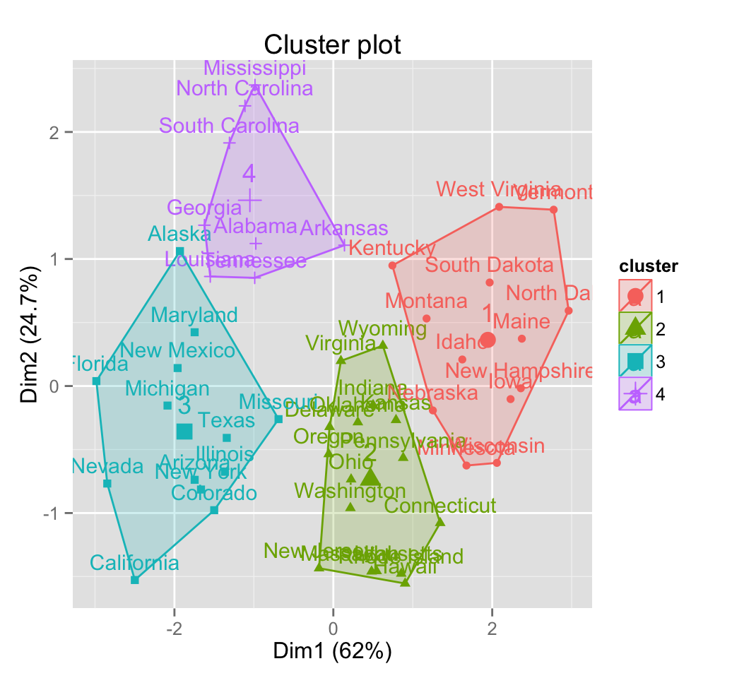
3 PAM: Partitioning Around Medoids
3.1 Concept
The use of means implies that k-means clustering is highly sensitive to outliers. This can severely affects the assignment of observations to clusters. A more robust algorithm is provided by PAM algorithm (Partitioning Around Medoids) which is also known as k-medoids clustering.
3.2 Algorithm
For a given cluster, the sum of the dissimilarities is calculated using Manhattan distance.
3.3 R function for computing PAM
The function pam() [in cluster package] and pamk() [in fpc package] can be used to compute PAM.
The function pamk() does not require a user to decide the number of clusters K.
In the following examples, well describe only the function pam(), which simplified format is:
pam(x, k)- x: possible values includes:
- Numeric data matrix or numeric data frame: each row corresponds to an observation, and each column corresponds to a variable.
- Dissimilarity matrix: in this case x is typically the output of daisy() or dist()
- k: The number of clusters
The function pam() has many features compared to the function kmeans():
- It accepts a dissimilarity matrix
- It is more robust to outliers because it uses medoids and it minimizes a sum of dissimilarities (based on Manhattan distance) instead of a sum of squared Euclidean distances.
- It provides a novel graphical display, the silhouette plot (see the function plot.partition())
3.4 Compute PAM
library("cluster")
# Load data
data("USArrests")
# Scale the data and compute pam with k = 4
pam.res <- pam(scale(USArrests), 4)
The function pam() returns an object of class pam which components include:
- medoids: Objects that represent clusters
- clustering: a vector containing the cluster number of each object
- Extract cluster medoids:
pam.res$medoids## Murder Assault UrbanPop Rape
## Alabama 1.2425641 0.7828393 -0.5209066 -0.003416473
## Michigan 0.9900104 1.0108275 0.5844655 1.480613993
## Oklahoma -0.2727580 -0.2371077 0.1699510 -0.131534211
## New Hampshire -1.3059321 -1.3650491 -0.6590781 -1.252564419The medoids are Alabama, Michigan, Oklahoma, New Hampshire
- Extract clustering vectors
head(pam.res$cluster)## Alabama Alaska Arizona Arkansas California Colorado
## 1 2 2 1 2 2The result can be plotted using the function clusplot() [in cluster package] as follow:
clusplot(pam.res, main = "Cluster plot, k = 4",
         color = TRUE)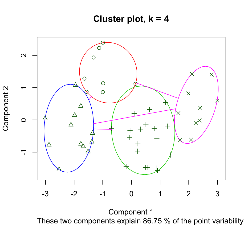
An alternative plot can be generated using the function fviz_cluster [in factoextra package]:
fviz_cluster(pam.res)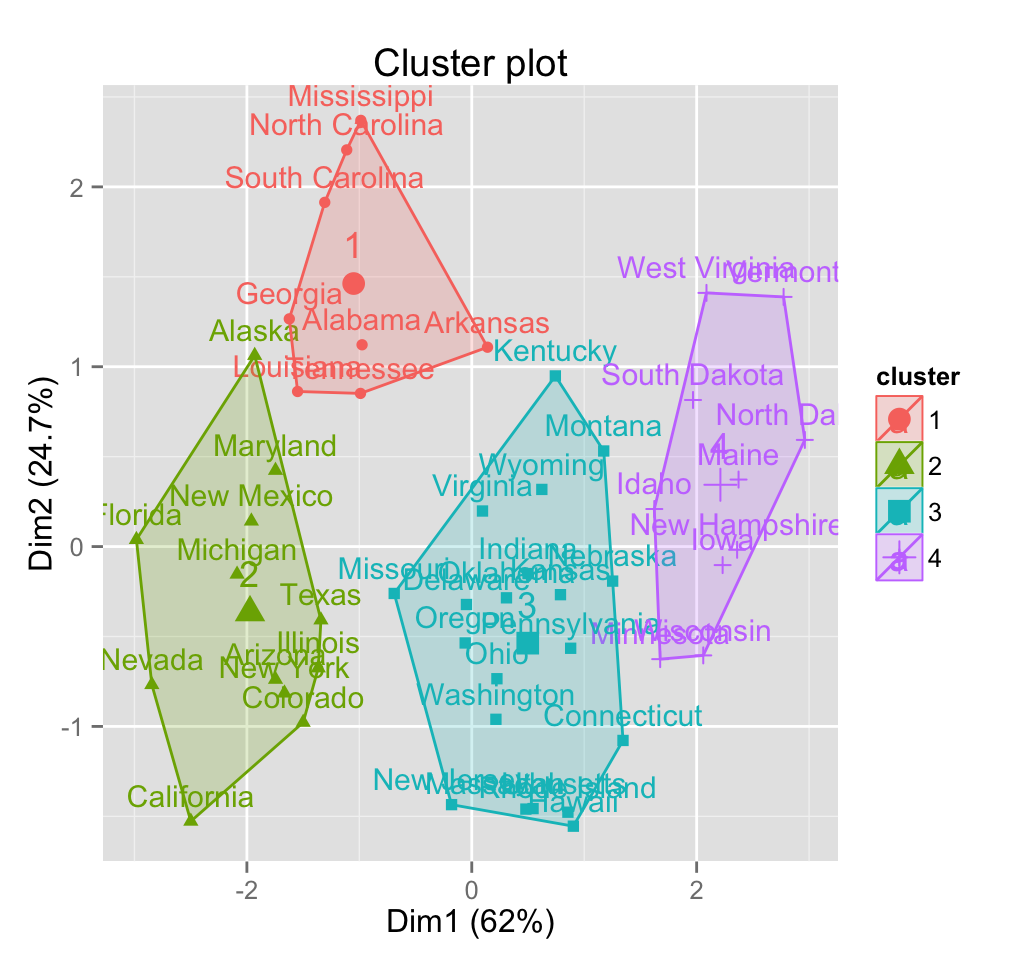
Its also possible to draw a silhouette plot as follow:
plot(silhouette(pam.res), col = 2:5) 
Silhouette Plot shows for each cluster:
- The number of elements (\(n_j\)) per cluster. Each horizontal line corresponds to an element. The length of the lines corresponds to silhouette width (\(S_i\)), which is the means similarity of each element to its own cluster minus the mean similarity to the next most similar cluster
- The average silhouette width
An alternative to draw silhouette plot is to use the function fviz_silhouette() [in factoextra]:
fviz_silhouette(silhouette(pam.res)) ## cluster size ave.sil.width
## 1 1 8 0.39
## 2 2 12 0.31
## 3 3 20 0.28
## 4 4 10 0.46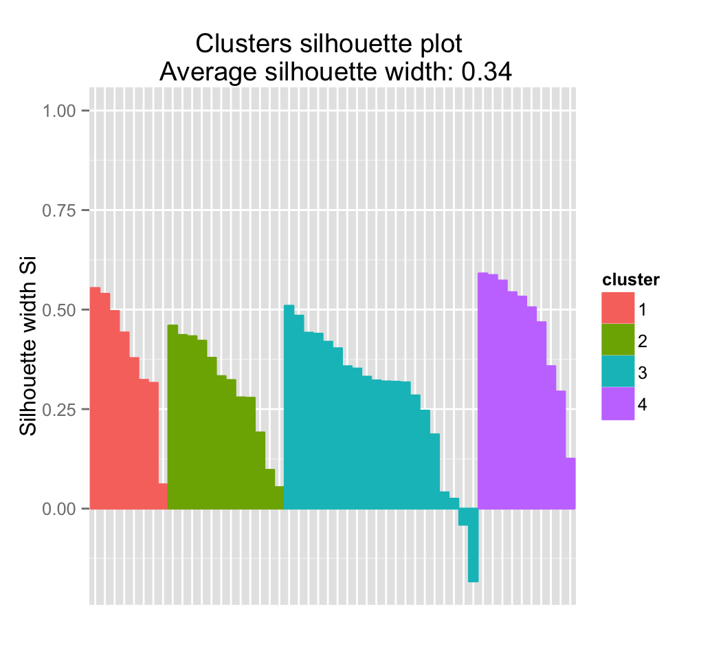
It can be seen that some samples have a negative silhouette. This means that they are not in the right cluster. We can find the name of these samples and determine the clusters they are closer, as follow:
# Compute silhouette
sil <- silhouette(pam.res)[, 1:3]
# Objects with negative silhouette
neg_sil_index <- which(sil[, 'sil_width'] < 0)
sil[neg_sil_index, , drop = FALSE]
## cluster neighbor sil_width
## Nebraska 3 4 -0.04034739
## Montana 3 4 -0.18266793Note that, for large datasets, pam() may need too much memory or too much computation time. In this case, the function clara() is preferable.
4 CLARA: Clustering Large Applications
4.1 Concept
CLARA is a partitioning method used to deal with much larger data sets (more than several thousand observations) in order to reduce computing time and RAM storage problem.
Note that, what can be considered small/large, is really a function of available computing power, both memory (RAM) and speed.
4.2 Algorithm
The algorithm is as follow:
- Split randomly the data sets in multiple subsets with fixed size
- Compute PAM algorithm on each subset and choose the corresponding k representative objects (medoids). Assign each observation of the entire dataset to the nearest medoid.
- Calculate the mean (or the sum) of the dissimilarities of the observations to their closest medoid. This is used as a measure of the goodness of the clustering.
- Retain the sub-dataset for which the mean (or sum) is minimal. A further analysis is carried out on the final partition.
4.3 R function for computing CLARA
The function clara() [in cluster package] can be used:
clara(x, k, samples = 5)- x: a numeric data matrix or data frame, each row corresponds to an observation, and each column corresponds to a variable.
- k: the number of cluster
- samples: number of samples to be drawn from the dataset. Default value is 5 but its recommended a much larger value.
clara() function can be used as follow:
set.seed(1234)
# Generate 500 objects, divided into 2 clusters.
x <- rbind(cbind(rnorm(200,0,8), rnorm(200,0,8)),
           cbind(rnorm(300,50,8), rnorm(300,50,8)))
head(x)
## [,1] [,2]
## [1,] -9.656526 3.881815
## [2,] 2.219434 5.574150
## [3,] 8.675529 1.484111
## [4,] -18.765582 5.605868
## [5,] 3.432998 2.493448
## [6,] 4.048447 6.083699# Compute clara
clarax <- clara(x, 2, samples=50)
# Cluster plot
fviz_cluster(clarax, stand = FALSE, geom = "point",
pointsize = 1)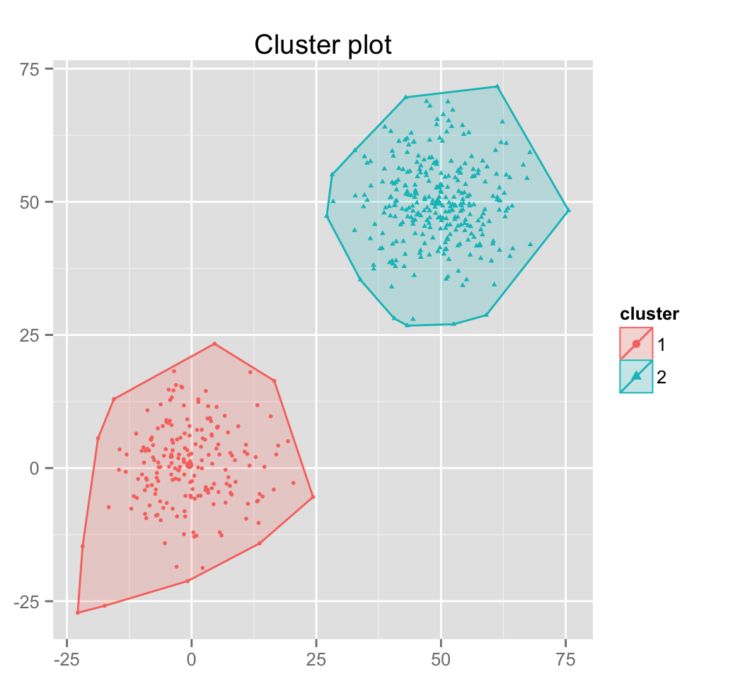
# Silhouette plot
plot(silhouette(clarax), col = 2:3, main = "Silhouette plot") 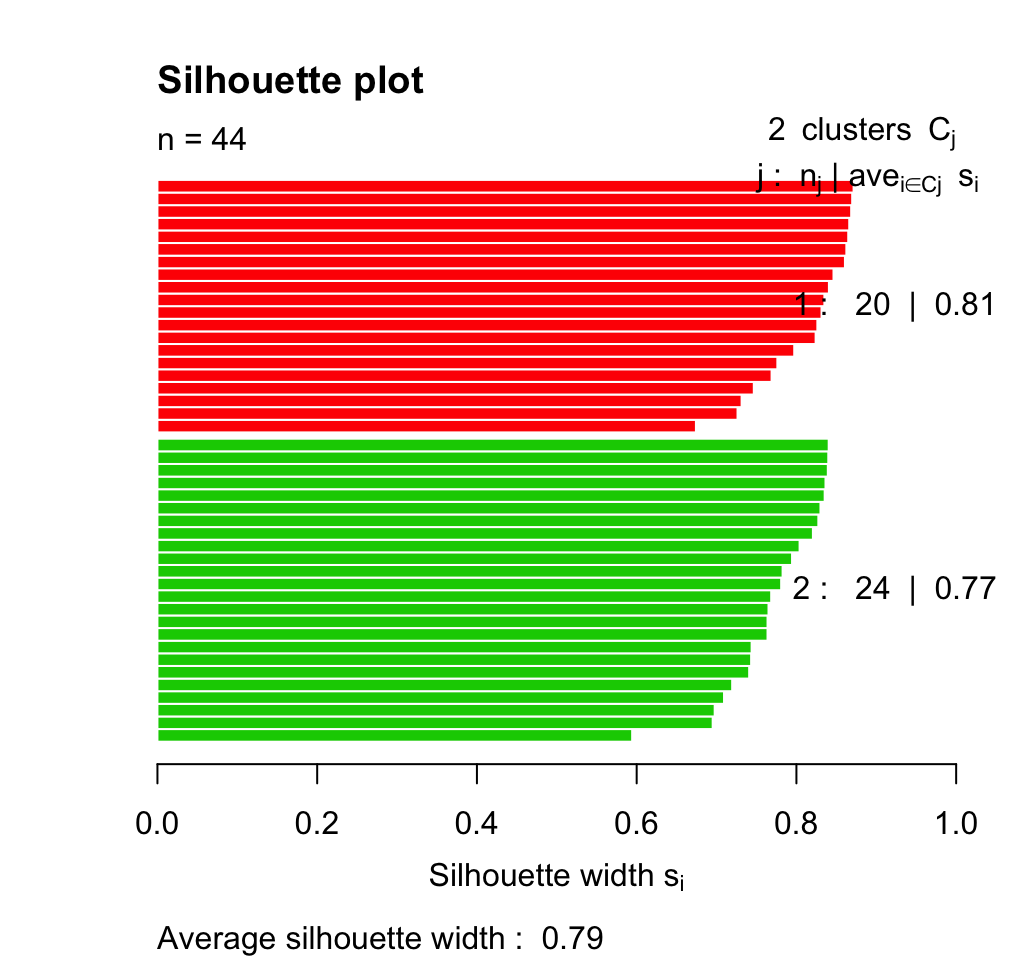
The output of the function clara() includes the following components:
- medoids: Objects that represent clusters
- clustering: a vector containing the cluster number of each object
- sample: labels or case numbers of the observations in the best sample, that is, the sample used by the clara algorithm for the final partition.
# Medoids
clarax$medoids
## [,1] [,2]
## [1,] -1.531137 1.145057
## [2,] 48.357304 50.233499# Clustering
head(clarax$clustering, 20)## [1] 1 1 1 1 1 1 1 1 1 1 1 1 1 1 1 1 1 1 1 15 R packages and functions for visualizing partitioning clusters
There are many functions from different packages for plotting cluster solutions generated by partitioning methods.
In this section, well describe the function clustplot() [in cluster package] and the function fviz_cluster() [in factoextra package]
With each of the above functions, a Principal Component Analysis is performed firstly and the observations are plotted according to the first two principal components.
5.1 clusplot() function
It creates a bivariate plot visualizing a partition of the data. All observations are represented by points in the plot, using principal components analysis. An ellipse is drawn around each cluster.
A simplified format is:
clustplot(x, clus, main = NULL, stand = FALSE, color = FALSE,
labels = 0)- x: an object of class partition created by one of the functions pam(), clara() or fanny()
- clus: a vector containing the cluster number to which each observation has been assigned
- stand: logical value: if TRUE the data will be standardized
- color: logical value: If TRUE, the ellipses are colored
- labels: possible values are 0, 1, 2, 3, 4 and 5
- labels = 0: no labels are placed in the plot
- labels = 2: all points and ellipses are labelled in the plot
- labels = 3: only the points are labelled in the plot
- labels = 4: only the ellipses are labelled in the plot
- col.p: color code(s) used for the observation points
- col.txt: color code(s) used for the labels (if labels >= 2)
- col.clus: color code for the ellipses (and their labels); only one if color is false (as per default).
set.seed(123)
# K-means clustering
km.res <- kmeans(scale(USArrests), 4, nstart = 25)
# Use clusplot function
library(cluster)
clusplot(scale(USArrests), km.res$cluster,  main = "Cluster plot",
         color=TRUE, labels = 2, lines = 0)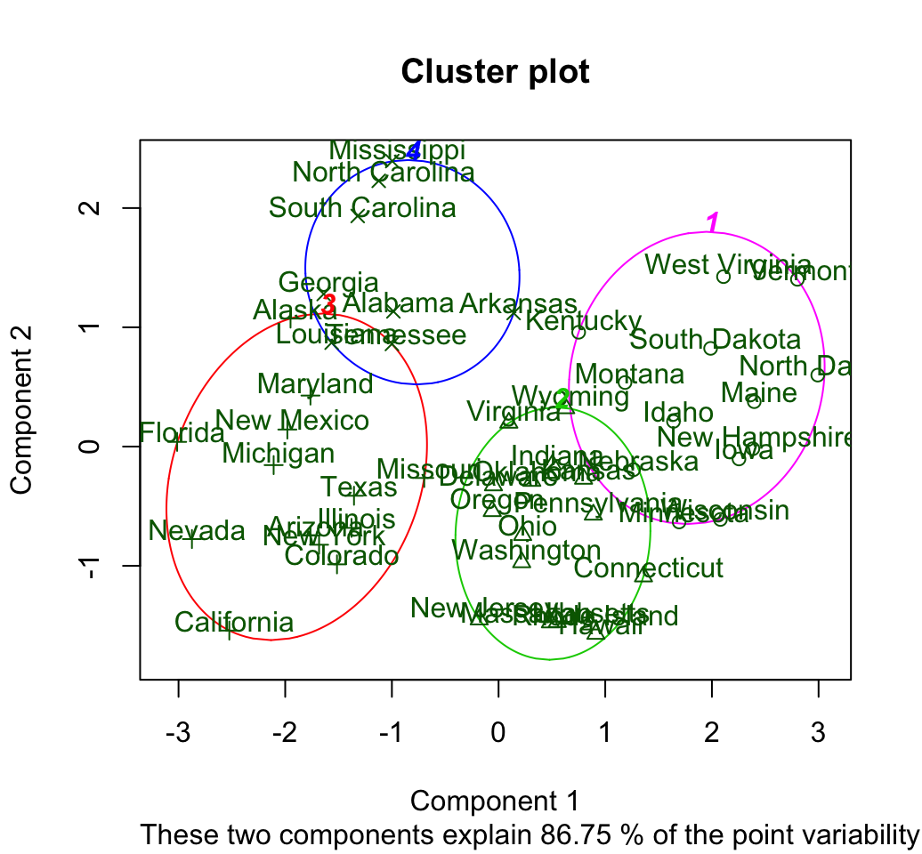
Its possible to generate the same plots for pam approach, as follow.
clusplot(pam.res, main = "Cluster plot, k = 4",
         color = TRUE)
5.2 fviz_cluster() function
The function fviz_cluster() [in factoextra package] can be used to draw clusters using ggplot2 plotting system.
Its possible to use it for visualizing the results of k-means, pam, clara and fanny.
A simplified format is:
fviz_cluster(object, data = NULL, stand = TRUE,
             geom = c("point", "text"),
frame = TRUE, frame.type = "convex")- object: an object of class partition created by the functions pam(), clara() or fanny() in cluster package. It can be also an output of kmeans() function in stats package. In this case the argument data is required.
- data: the data that has been used for clustering. Required only when object is a class of kmeans.
- stand: logical value; if TRUE, data is standardized before principal component analysis
- geom: a text specifying the geometry to be used for the graph. Allowed values are the combination of c(point, text). Use point (to show only points); text to show only labels; c(point, text) to show both types.
- frame: logical value; if TRUE, draws outline around points of each cluster
- frame.type: Character specifying frame type. Possible values are convex or types supported by ggplot2::stat_ellipse including one of c(t, norm, euclid).
In order to use the function fviz_cluster(), make sure that the package factoextra is installed and loaded.
library("factoextra")
# Visualize kmeans clustering
fviz_cluster(km.res, USArrests)
# Visualize pam clustering
pam.res <- pam(scale(USArrests), 4)
fviz_cluster(pam.res)
# Change frame type
fviz_cluster(pam.res, frame.type = "t")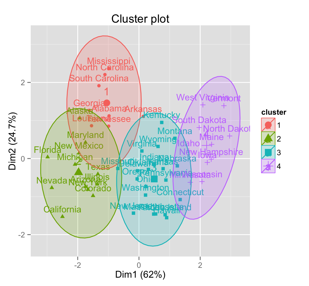
# Remove ellipse fill color
# Change frame level
fviz_cluster(pam.res, frame.type = "t",
             frame.alpha = 0, frame.level = 0.7)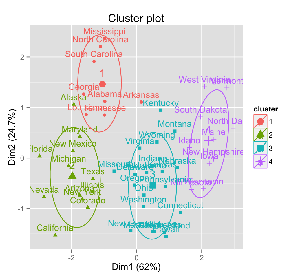
# Show point only
fviz_cluster(pam.res, geom = "point")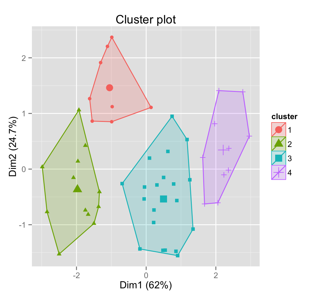
# Show text only
fviz_cluster(pam.res, geom = "text")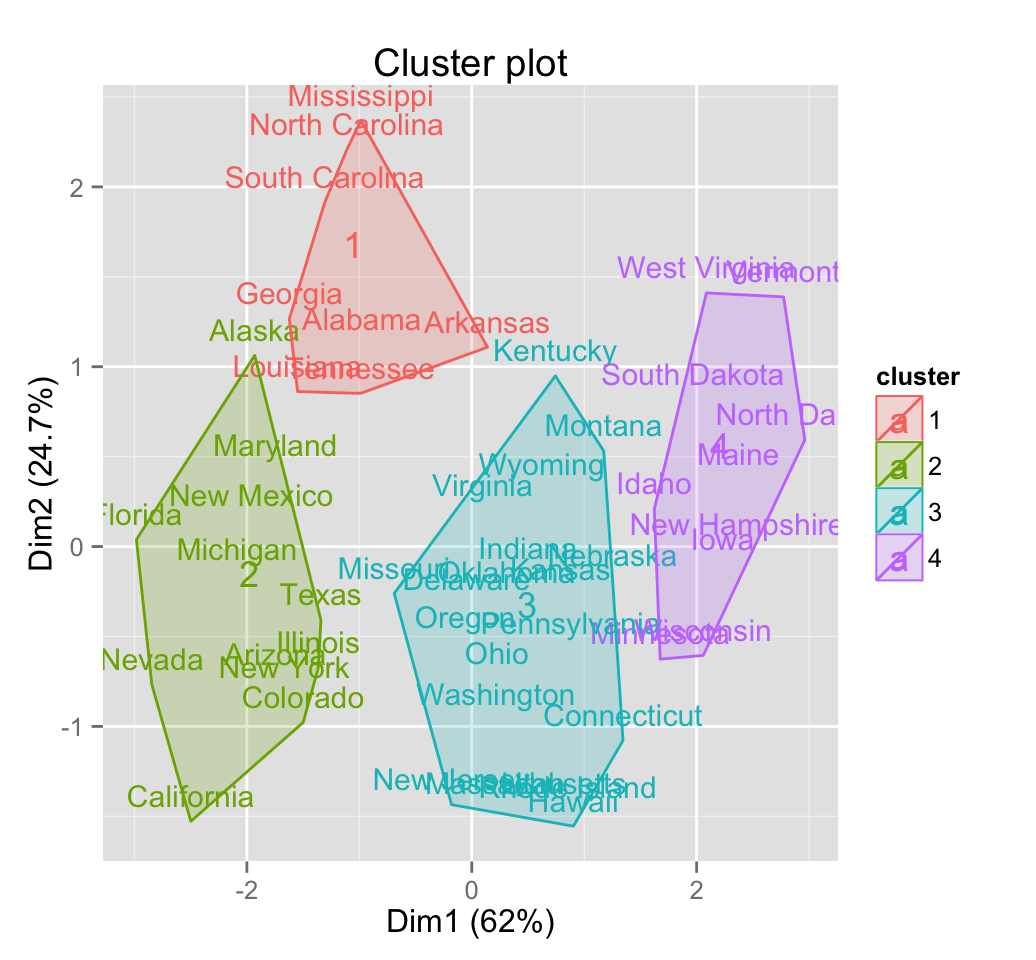
# Change the color and theme
fviz_cluster(pam.res) +
  scale_color_brewer(palette = "Set2")+
  scale_fill_brewer(palette = "Set2") +
  theme_minimal()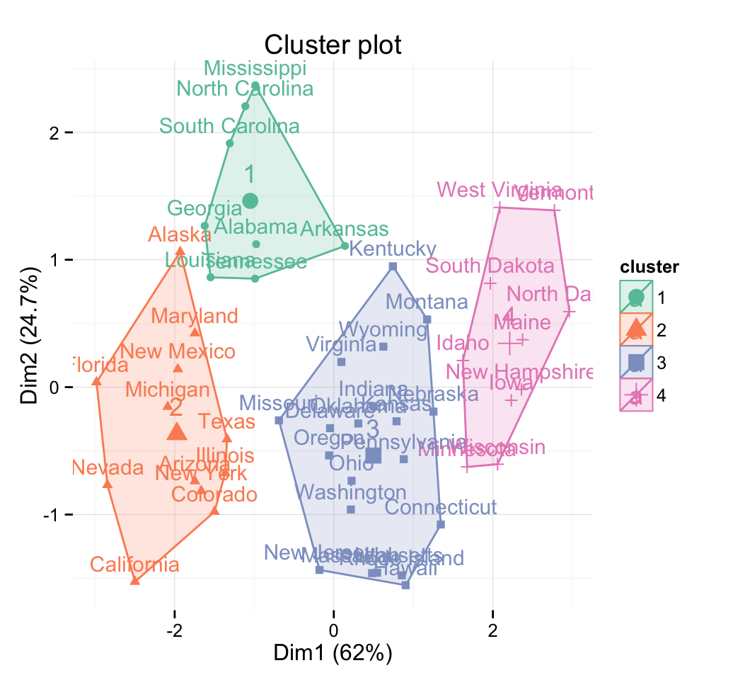
6 Infos
This analysis has been performed using R software (ver. 3.2.1)
- Hartigan, J. A. and Wong, M. A. (1979). A K-means clustering algorithm. Applied Statistics 28, 100108.
- Kaufman, L. and Rousseeuw, P.J. (1990). Finding Groups in Data: An Introduction to Cluster Analysis. Wiley, New York.
- MacQueen, J. (1967) Some methods for classification and analysis of multivariate observations. In Proceedings of the Fifth Berkeley Symposium on Mathematical Statistics and Probability, eds L. M. Le Cam & J. Neyman, 1, pp. 281297. Berkeley, CA: University of California Press.