1 Concept

The traditional clustering methods such as hierarchical clustering and partitioning algorithms (k-means and others) are heuristic and are not based on formal models.

An alternative is to use model-based clustering, in which, the data are considered as coming from a distribution that is mixture of two or more components (i.e. clusters) (Chris Fraley and Adrian E. Raftery, 2002 and 2012).

Each component k (i.e. group or cluster) is modeled by the normal or Gaussian distribution which is characterized by the parameters:

• \(\mu_k\): mean vector,
• \(\sum_k\): covariance matrix,
• An associated probability in the mixture. Each point has a probability of belonging to each cluster.

2 Model parameters

The model parameters can be estimated using the EM (Expectation-Maximization) algorithm initialized by hierarchical model-based clustering. Each cluster k is centered at the means \(\mu_k\), with increased density for points near the mean.

Geometric features (shape, volume, orientation) of each cluster are determined by the covariance matrix \(\sum_k\).

Different possible parameterizations of \(\sum_k\) are available in the R package mclust (see ?mclustModelNames).

The available model options, in mclust package, are represented by identifiers including: EII, VII, EEI, VEI, EVI, VVI, EEE, EEV, VEV and VVV.

The first identifier refers to volume, the second to shape and the third to orientation. E stands for “equal”, V for “variable” and I for “coordinate axes”.

For example:

• EVI denotes a model in which the volumes of all clusters are equal (E), the shapes of the clusters may vary (V), and the orientation is the identity (I) or “coordinate axes.
  
• EEE means that the clusters have the same volume, shape and orientation in p-dimensional space.
• VEI means that the clusters have variable volume, the same shape and orientation equal to coordinate axes.

The mclust package uses maximum likelihood to fit all these models, with different covariance matrix parameterizations, for a range of k components. The “best model” is selected using the Bayesian Information Criterion or BIC. A large BIC score indicates strong evidence for the corresponding model.

3 Advantage of model-based clustering

The key advantage of model-based approach, compared to the standard clustering methods (k-means, hierarchical clustering, …), is the suggestion of the number of clusters and an appropriate model.

4 Example of data

We’ll use the bivariate faithful data set which contains the waiting time between eruptions and the duration of the eruption for the Old Faithful geyser in Yellowstone National Park (Wyoming, USA).

# Load the data
data("faithful")
head(faithful)

##   eruptions waiting
## 1     3.600      79
## 2     1.800      54
## 3     3.333      74
## 4     2.283      62
## 5     4.533      85
## 6     2.883      55

An illustration of the data can be drawn using ggplot2 package as follow:

library("ggplot2")
ggplot(faithful, aes(x=eruptions, y=waiting)) +
  geom_point() +  # Scatter plot
  geom_density2d() # Add 2d density estimation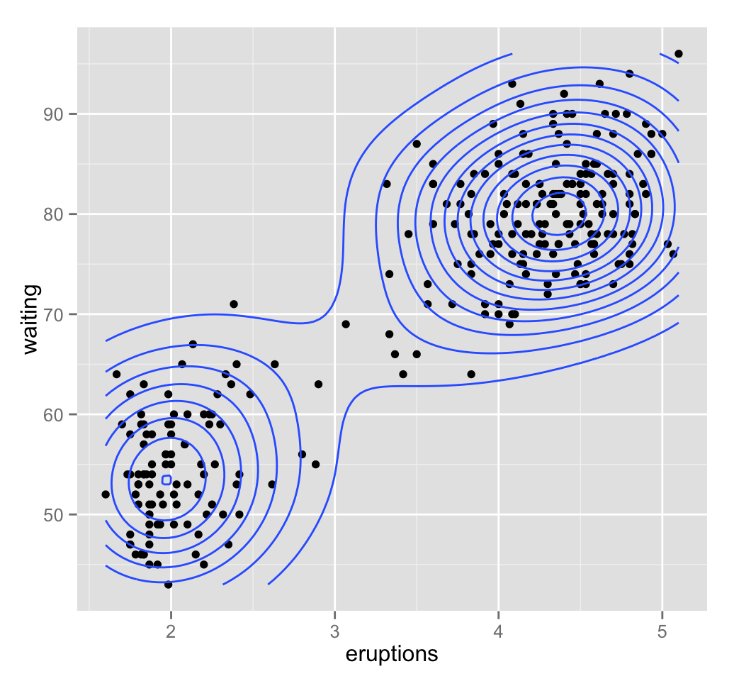

5 Mclust(): R function for computing model-based clustering

The function Mclust() [in mclust package] can be used to compute model-based clustering.

Install and load the package as follow:

# Install
install.packages("mclust")

# Load
library("mclust")

The function Mclust() provides the optimal mixture model estimation according to BIC. A simplified format is:

Mclust(data, G = NULL)

The function Mclust() returns an object of class ‘Mclust’ containing the following elements:

• modelName: A character string denoting the model at which the optimal BIC occurs.
• G: The optimal number of mixture components (i.e: number of clusters)
• BIC: All BIV values
• bic Optimal BIC value
• loglik: The loglikelihood corresponding to the optimal BIC
• df: The number of estimated parameters
• Z: A matrix whose \([i,k]^{th}\) entry is the probability that observation \(i\) in the test data belongs to the \(k^{th}\) class. Column names are cluster numbers, and rows are observations
• classification: The cluster number of each observation, i.e. map(z)
• uncertainty: The uncertainty associated with the classification

6 Example of cluster analysis using Mclust()

library(mclust)
# Model-based-clustering
mc <- Mclust(faithful)
# Print a summary
summary(mc)

## ----------------------------------------------------
## Gaussian finite mixture model fitted by EM algorithm 
## ----------------------------------------------------
## 
## Mclust EEE (ellipsoidal, equal volume, shape and orientation) model with 3 components:
## 
##  log.likelihood   n df       BIC       ICL
##       -1126.361 272 11 -2314.386 -2360.865
## 
## Clustering table:
##   1   2   3 
## 130  97  45

# Values returned by Mclust()
names(mc)

##  [1] "call"           "data"           "modelName"      "n"             
##  [5] "d"              "G"              "BIC"            "bic"           
##  [9] "loglik"         "df"             "hypvol"         "parameters"    
## [13] "z"              "classification" "uncertainty"

# Optimal selected model
mc$modelName

## [1] "EEE"

# Optimal number of cluster
mc$G

## [1] 3

# Probality for an observation to be in a given cluster
head(mc$z)

##           [,1]         [,2]         [,3]
## 1 2.181744e-02 1.130837e-08 9.781825e-01
## 2 2.475031e-21 1.000000e+00 3.320864e-13
## 3 2.521625e-03 2.051823e-05 9.974579e-01
## 4 6.553336e-14 9.999998e-01 1.664978e-07
## 5 9.838967e-01 7.642900e-20 1.610327e-02
## 6 2.104355e-07 9.975388e-01 2.461029e-03

# Cluster assignement of each observation
head(mc$classification, 10)

##  1  2  3  4  5  6  7  8  9 10 
##  3  2  3  2  1  2  1  3  2  1

# Uncertainty associated with the classification
head(mc$uncertainty)

##            1            2            3            4            5 
## 2.181745e-02 3.321787e-13 2.542143e-03 1.664978e-07 1.610327e-02 
##            6 
## 2.461239e-03

Model-based clustering results can be drawn using the function plot.Mclust():

plot(x, what = c("BIC", "classification", "uncertainty", "density"),
     xlab = NULL, ylab = NULL, addEllipses = TRUE, main = TRUE, ...)

# BIC values used for choosing the number of clusters
plot(mc, "BIC")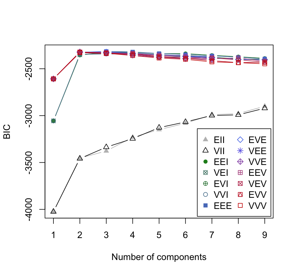

# Classification: plot showing the clustering
plot(mc, "classification")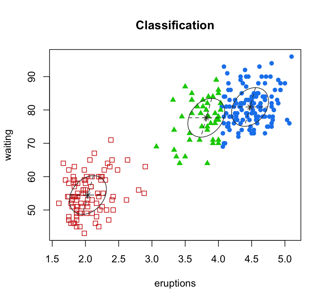

# Classification uncertainty
plot(mc, "uncertainty")

# Estimated density. Contour plot
plot(mc, "density")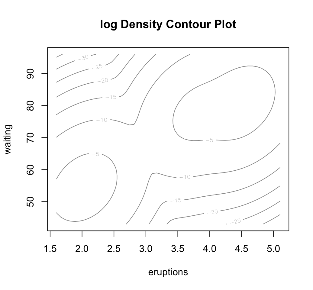

Clusters generated by Mclust() can be drawn using the function fviz_cluster() [in factoextra package]. Read more about [factoextra](http://www.sthda.com/english/wiki/factoextra-r-package-quick-multivariate-data-analysis-pca-ca-mca-and-visualization-r-software-and-data-mining.

library(factoextra)
fviz_cluster(mc, frame.type = "norm", geom = "point")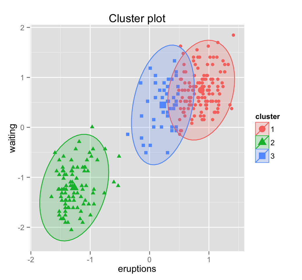

7 Infos

This analysis has been performed using R software (ver. 3.2.3)

• Chris Fraley, A. E. Raftery, T. B. Murphy and L. Scrucca (2012). mclust Version 4 for R: Normal Mixture Modeling for Model-Based Clustering, Classification, and Density Estimation. Technical Report No. 597, Department of Statistics, University of Washington. pdf
• Chris Fraley and A. E. Raftery (2002). Model-based clustering, discriminant analysis, and density estimation. Journal of the American Statistical Association 97:611:631.