Humans abilities are exceeded by the large amounts of data collected every day from different fields, bio-medical, security, marketing, web search, geo-spatial or other automatic equipment. Consequently, unsupervised machine learning technics, such as clustering, are used for discovering knowledge from big data.
Clustering approaches classify samples into groups (i.e clusters) containing objects of similar profiles. In our previous post, we clarified distance measures for assessing similarity between observations.
In this chapter well describe the different steps to follow for computing clustering on a real data using k-means clustering:
1 Required packages
The following packages will be used:
- cluster for clustering analyses
- factoextra for visualizing clusters using ggplot2 plotting system
Install factoextra package as follow:
if(!require(devtools)) install.packages("devtools")
devtools::install_github("kassambara/factoextra")
The cluster package can be installed using the code below:
install.packages("cluster")Load packages:
library(cluster)
library(factoextra)
2 Data preparation
Well use the built-in R data set USArrests, which can be loaded and prepared as follow:
# Load the data set
data(USArrests)

# Remove any missing value (i.e, NA values for not available)
# That might be present in the data
USArrests <- na.omit(USArrests)

# View the firt 6 rows of the data
head(USArrests, n = 6)
## Murder Assault UrbanPop Rape
## Alabama 13.2 236 58 21.2
## Alaska 10.0 263 48 44.5
## Arizona 8.1 294 80 31.0
## Arkansas 8.8 190 50 19.5
## California 9.0 276 91 40.6
## Colorado 7.9 204 78 38.7In this data set, columns are variables and rows are observations (i.e., samples).
To inspect the data before the K-means clustering well compute some descriptive statistics such as the mean and the standard deviation of the variables.
The apply() function is used to apply a given function (e.g : min(), max(), mean(), ) on the data set. The second argument can take the value of:
- 1: for applying the function on the rows
- 2: for applying the function on the columns
desc_stats <- data.frame(
  Min = apply(USArrests, 2, min), # minimum
  Med = apply(USArrests, 2, median), # median
  Mean = apply(USArrests, 2, mean), # mean
  SD = apply(USArrests, 2, sd), # Standard deviation
  Max = apply(USArrests, 2, max) # Maximum
  )
desc_stats <- round(desc_stats, 1)
head(desc_stats)
## Min Med Mean SD Max
## Murder 0.8 7.2 7.8 4.4 17.4
## Assault 45.0 159.0 170.8 83.3 337.0
## UrbanPop 32.0 66.0 65.5 14.5 91.0
## Rape 7.3 20.1 21.2 9.4 46.0Note that the variables have a large different means and variances. They must be standardized to make them comparable.
Standardization consists of transforming the variables such that they have mean zero and standard deviation one. The scale() function can be used as follow:
df<- scale(USArrests)3 Assessing the clusterability
The function get_clust_tendency() [in factoextra] can be used. It computes Hopkins statistic and provides a visual approach.
library("factoextra")
res <- get_clust_tendency(df, 40, graph = FALSE)
# Hopskin statistic
res$hopkins_stat
## [1] 0.3440875# Visualize the dissimilarity matrix
res$plot## NULLThe value of Hopkins statistic is significantly < 0.5, indicating that the data is highly clusterable. Additionally, It can be seen that the ordered dissimilarity image contains patterns (i.e., clusters).
4 Estimate the number of clusters in the data
As k-means clustering requires to specify the number of clusters to generate, well use the function clusGap() [in cluster] to compute gap statistics for estimating the optimal number of clusters . The function fviz_gap_stat() [in factoextra] is used to visualize the gap statistic plot.
library("cluster")
set.seed(123)
# Compute the gap statistic
gap_stat <- clusGap(df, FUN = kmeans, nstart = 25,
                    K.max = 10, B = 500)
# Plot the result
library(factoextra)
fviz_gap_stat(gap_stat)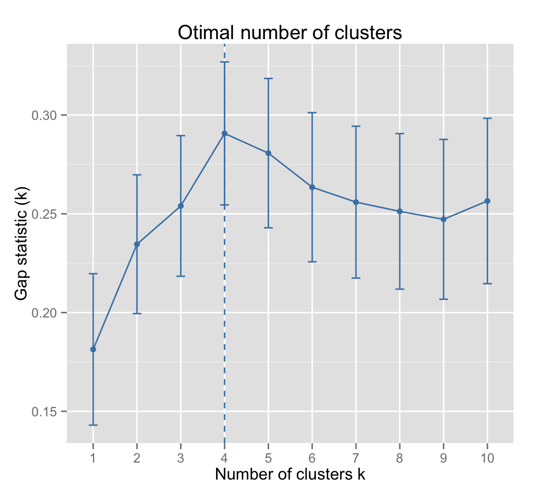
The gap statistic suggests a 4 cluster solutions.
Its also possible to use the function NbClust() [in NbClust] package.
5 Compute k-means clustering
K-means clustering with k = 4:
# Compute k-means
set.seed(123)
km.res <- kmeans(df, 4, nstart = 25)
head(km.res$cluster, 20)
## Alabama Alaska Arizona Arkansas California Colorado
## 4 3 3 4 3 3
## Connecticut Delaware Florida Georgia Hawaii Idaho
## 2 2 3 4 2 1
## Illinois Indiana Iowa Kansas Kentucky Louisiana
## 3 2 1 2 1 4
## Maine Maryland
## 1 3# Visualize clusters using factoextra
fviz_cluster(km.res, USArrests)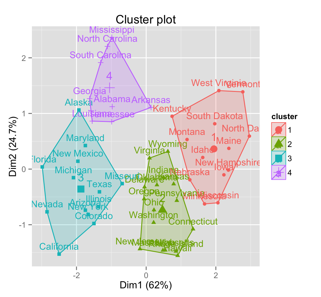
6 Cluster validation statistics: Inspect cluster silhouette plot
Recall that the silhouette measures (\(S_i\)) how similar an object \(i\) is to the the other objects in its own cluster versus those in the neighbor cluster. \(S_i\) values range from 1 to - 1:
- A value of \(S_i\) close to 1 indicates that the object is well clustered. In the other words, the object \(i\) is similar to the other objects in its group.
- A value of \(S_i\) close to -1 indicates that the object is poorly clustered, and that assignment to some other cluster would probably improve the overall results.
sil <- silhouette(km.res$cluster, dist(df))
rownames(sil) <- rownames(USArrests)
head(sil[, 1:3])
## cluster neighbor sil_width
## Alabama 4 3 0.48577530
## Alaska 3 4 0.05825209
## Arizona 3 2 0.41548326
## Arkansas 4 2 0.11870947
## California 3 2 0.43555885
## Colorado 3 2 0.32654235fviz_silhouette(sil)## cluster size ave.sil.width
## 1 1 13 0.37
## 2 2 16 0.34
## 3 3 13 0.27
## 4 4 8 0.39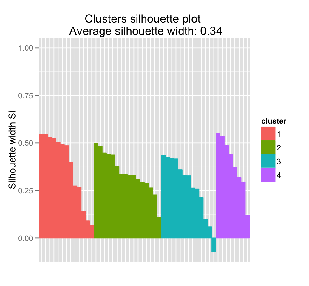
It can be seen that there are some samples which have negative silhouette values. Some natural questions are :
Which samples are these? To what cluster are they closer?
This can be determined from the output of the function silhouette() as follow:
neg_sil_index <- which(sil[, "sil_width"] < 0)
sil[neg_sil_index, , drop = FALSE]
## cluster neighbor sil_width
## Missouri 3 2 -0.073181447 eclust(): Enhanced clustering analysis
The function eclust() [in factoextra] provides several advantages compared to the standard packages used for clustering analysis:
- It simplifies the workflow of clustering analysis
- It can be used to compute hierarchical clustering and partitioning clustering in a single line function call
- The function eclust() computes automatically the gap statistic for estimating the right number of clusters.
- It automatically provides silhouette information
- It draws beautiful graphs using ggplot2
7.1 K-means clustering using eclust()
# Compute k-means
res.km <- eclust(df, "kmeans")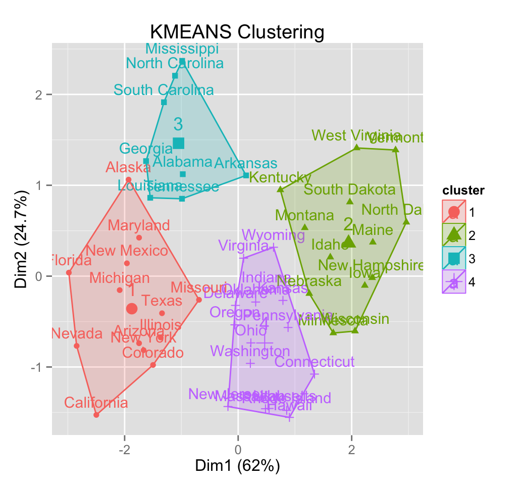
# Gap statistic plot
fviz_gap_stat(res.km$gap_stat)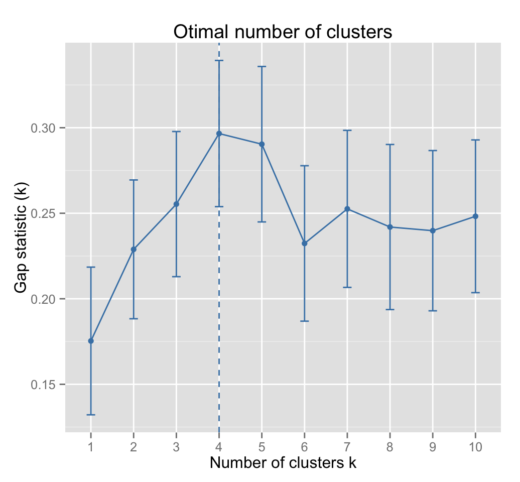
# Silhouette plot
fviz_silhouette(res.km)
## cluster size ave.sil.width
## 1 1 13 0.27
## 2 2 13 0.37
## 3 3 8 0.39
## 4 4 16 0.34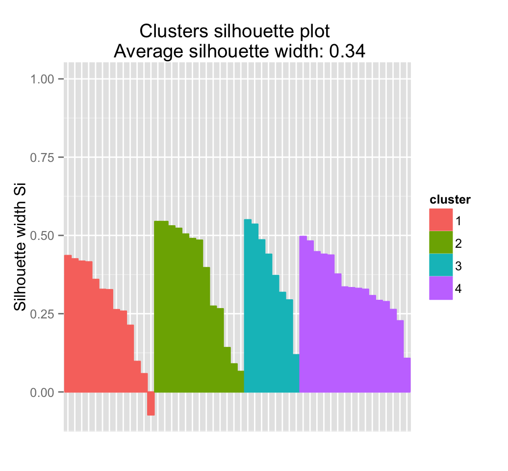
7.2 Hierachical clustering using eclust()
 # Enhanced hierarchical clustering
res.hc <- eclust(df, "hclust") # compute hclust
fviz_dend(res.hc, rect = TRUE) # dendrogam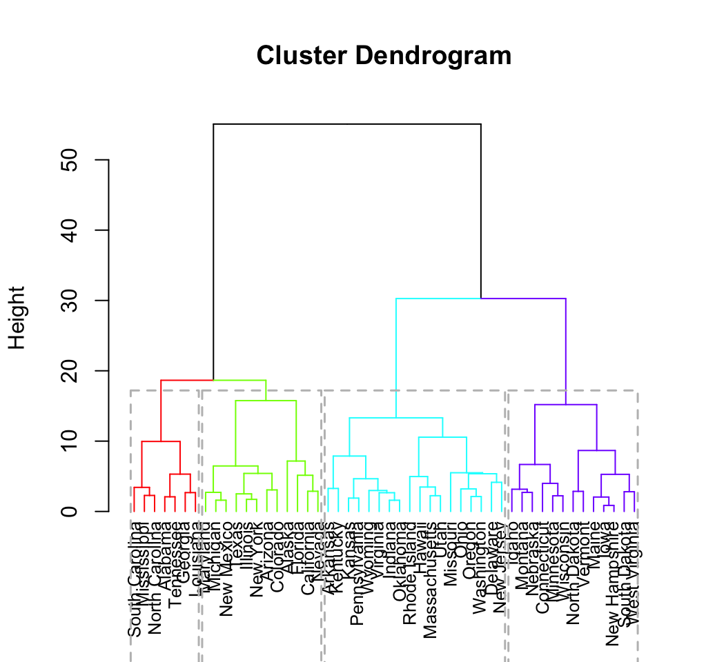
The R code below generates the silhouette plot and the scatter plot for hierarchical clustering.
fviz_silhouette(res.hc) # silhouette plot
fviz_cluster(res.hc) # scatter plot
8 Infos
This analysis has been performed using R software (ver. 3.2.3)