1 Required packages
Three R packages are required for this chapter:
- cluster and e1071 for computing fuzzy clustering
- factoextra for visualizing clusters
install.packages("cluster")
install.packages("e1071")
install.packages("factoextra")
2 Concept of fuzzy clustering
In K-means or PAM clustering, the data is divided into distinct clusters, where each element is affected exactly to one cluster. This type of clustering is also known as hard clustering or non-fuzzy clustering. Unlike K-means, Fuzzy clustering is considered as a soft clustering, in which each element has a probability of belonging to each cluster. In other words, each element has a set of membership coefficients corresponding to the degree of being in a given cluster.
Points close to the center of a cluster, may be in the cluster to a higher degree than points in the edge of a cluster. The degree, to which an element belongs to a given cluster, is a numerical value in [0, 1].
Fuzzy c-means (FCM) algorithm is one of the most widely used fuzzy clustering algorithms. It was developed by Dunn in 1973 and improved by Bezdek in 1981. Its frequently used in pattern recognition.
3 Algorithm of fuzzy clustering
FCM algorithm is very similar to the k-means algorithm and the aim is to minimize the objective function defined as follow:
\[ \sum\limits_{j=1}^k \sum\limits_{x_i \in C_j} u_{ij}^m (x_i - \mu_j)^2 \]
Where,
- \(u_{ij}\) is the degree to which an observation \(x_i\) belongs to a cluster \(c_j\)
- \(\mu_j\) is the center of the cluster j
- \(u_{ij}\) is the degree to which an observation \(x_i\) belongs to a cluster \(c_j\)
- \(m\) is the fuzzifier.
It can be seen that, FCM differs from k-means by using the membership values \(u_{ij}\) and the fuzzifier \(m\).
The variable \(u_{ij}^m\) is defined as follow:
\[ u_{ij}^m = \frac{1}{\sum\limits_{l=1}^k \left( \frac{| x_i - c_j |}{| x_i - c_k |}\right)^{\frac{2}{m-1}}} \]
The degree of belonging, \(u_{ij}\), is linked inversely to the distance from x to the cluster center.
The parameter \(m\) is a real number greater than 1 (\(1.0 < m < \infty\)) and it defines the level of cluster fuzziness. Note that, a value of \(m\) close to 1 gives a cluster solution which becomes increasingly similar to the solution of hard clustering such as k-means; whereas a value of \(m\) close to infinite leads to complete fuzzyness.
Note that, a good choice is to use m = 2.0 (Hathaway and Bezdek 2001).
In fuzzy clustering the centroid of a cluster is he mean of all points, weighted by their degree of belonging to the cluster:
\[ C_j = \frac{\sum\limits_{x \in C_j} u_{ij}^m x}{\sum\limits_{x \in C_j} u_{ij}^m} \]
Where,
- \(C_j\) is the centroid of the cluster j
- \(u_{ij}\) is the degree to which an observation \(x_i\) belongs to a cluster \(c_j\)
The algorithm of fuzzy clustering can be summarize as follow:
- Specify a number of clusters k (by the analyst)
- Assign randomly to each point coefficients for being in the clusters.
- Repeat until the maximum number of iterations (given by maxit) is reached, or when the algorithm has converged (that is, the coefficients change between two iterations is no more than \(\epsilon\), the given sensitivity threshold):
- Compute the centroid for each cluster, using the formula above.
- For each point, compute its coefficients of being in the clusters, using the formula above.
The algorithm minimizes intra-cluster variance as well, but has the same problems as k-means; the minimum is a local minimum, and the results depend on the initial choice of weights. Hence, different initializations may lead to different results.
Using a mixture of Gaussians along with the expectation-maximization algorithm is a more statistically formalized method which includes some of these ideas: partial membership in classes.
3.1 R functions for fuzzy clustering
3.1.1 fanny(): Fuzzy analysis clustering
The function fanny() [in cluster package] can be used to compute fuzzy clustering. FANNY stands for fuzzy analysis clustering. A simplified format is:
fanny(x, k, memb.exp = 2, metric = "euclidean",
stand = FALSE, maxit = 500)- x: A data matrix or data frame or dissimilarity matrix
- k: The desired number of clusters to be generated
- memb.exp: The membership exponent (strictly larger than 1) used in the fit criteria. Its also known as the fuzzifier
- metric: The metric to be used for calculating dissimilarities between observations
- stand: Logical; if true, the measurements in x are standardized before calculating the dissimilarities
- maxit: maximal number of iterations
The function fanny() returns an object including the following components:
- membership: matrix containing the degree to which each observation belongs to a given cluster. Column names are the clusters and rows are observations
- coeff: Dunns partition coefficient F(k) of the clustering, where k is the number of clusters. F(k) is the sum of all squared membership coefficients, divided by the number of observations. Its value is between 1/k and 1. The normalized form of the coefficient is also given. It is defined as \((F(k) - 1/k) / (1 - 1/k)\), and ranges between 0 and 1. A low value of Dunns coefficient indicates a very fuzzy clustering, whereas a value close to 1 indicates a near-crisp clustering.
- clustering: the clustering vector containing the nearest crisp grouping of observations
A subset of USArrests data is used in the following example:
library(cluster)
set.seed(123)
# Load the data
data("USArrests")

# Subset of USArrests
ss <- sample(1:50, 20)
df <- scale(USArrests[ss,])

# Compute fuzzy clustering
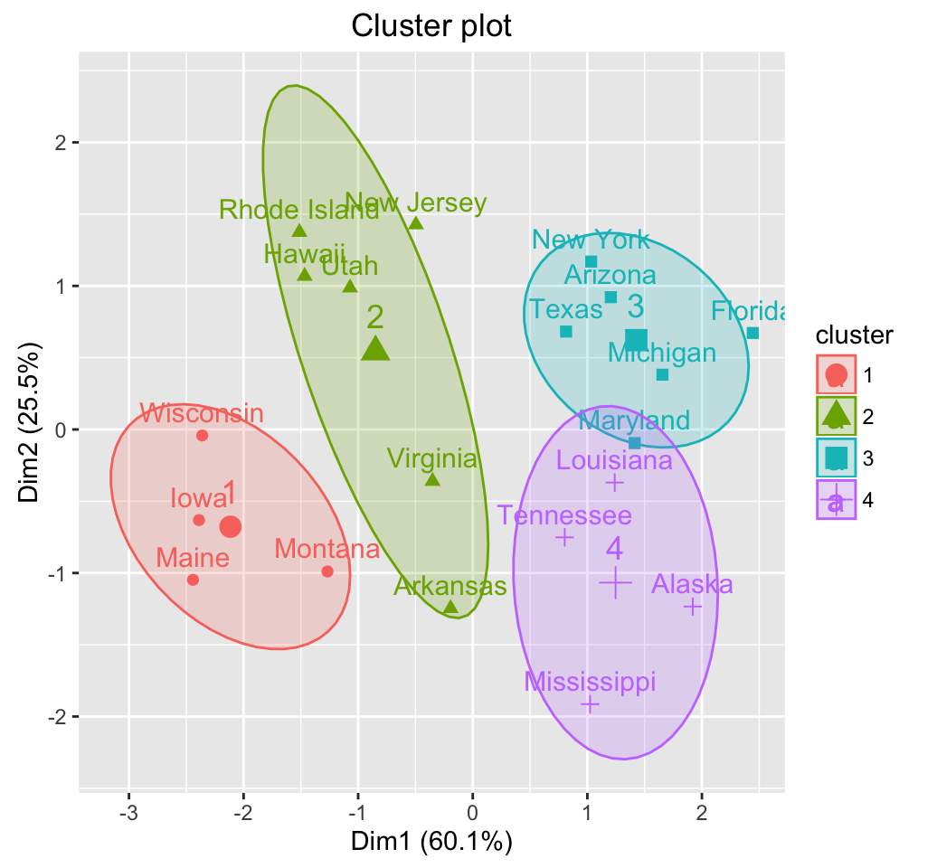
res.fanny <- fanny(df, 4)

# Cluster plot using fviz_cluster()
# You can use also : clusplot(res.fanny)
library(factoextra)
fviz_cluster(res.fanny, frame.type = "norm",
             frame.level = 0.68)
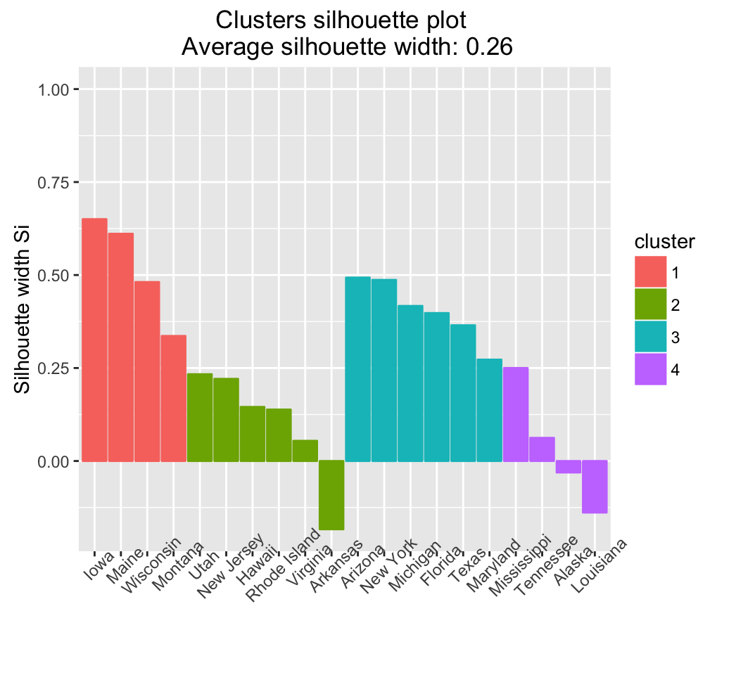
# Silhouette plot
fviz_silhouette(res.fanny, label = TRUE)
## cluster size ave.sil.width
## 1 1 4 0.52
## 2 2 6 0.10
## 3 3 6 0.41
## 4 4 4 0.04
The result of fanny() function can be printed as follow:
print(res.fanny)## Fuzzy Clustering object of class 'fanny' :
## m.ship.expon. 2
## objective 6.052789
## tolerance 1e-15
## iterations 215
## converged 1
## maxit 500
## n 20
## Membership coefficients (in %, rounded):
## [,1] [,2] [,3] [,4]
## Iowa 75 11 7 7
## Rhode Island 26 32 21 21
## Maryland 8 19 37 37
## Tennessee 10 24 33 33
## Utah 23 36 20 20
## Arizona 10 23 34 34
## Mississippi 16 25 29 29
## Wisconsin 65 15 10 10
## Virginia 17 37 23 23
## Maine 63 15 11 11
## Texas 8 25 33 33
## Louisiana 9 22 35 35
## Montana 41 26 17 17
## Michigan 8 20 36 36
## Arkansas 19 30 25 25
## New York 9 24 34 34
## Florida 10 21 35 35
## Alaska 15 24 31 31
## Hawaii 27 34 20 20
## New Jersey 16 37 23 23
## Fuzzyness coefficients:
## dunn_coeff normalized
## 0.31337355 0.08449807
## Closest hard clustering:
## Iowa Rhode Island Maryland Tennessee Utah
## 1 2 3 4 2
## Arizona Mississippi Wisconsin Virginia Maine
## 3 4 1 2 1
## Texas Louisiana Montana Michigan Arkansas
## 3 4 1 3 2
## New York Florida Alaska Hawaii New Jersey
## 3 3 4 2 2
##
## Available components:
## [1] "membership" "coeff" "memb.exp" "clustering" "k.crisp"
## [6] "objective" "convergence" "diss" "call" "silinfo"
## [11] "data"The different components can be extracted using the code below:
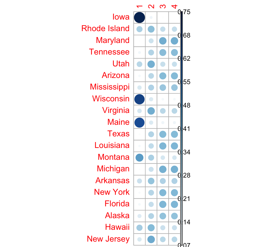
# Membership coefficient
res.fanny$membership
## [,1] [,2] [,3] [,4]
## Iowa 0.75234997 0.1056742 0.07098791 0.07098791
## Rhode Island 0.26129280 0.3198982 0.20940449 0.20940449
## Maryland 0.07559096 0.1906031 0.36690296 0.36690296
## Tennessee 0.10351700 0.2444743 0.32600436 0.32600436
## Utah 0.23177048 0.3631831 0.20252321 0.20252321
## Arizona 0.09505979 0.2329621 0.33598906 0.33598906
## Mississippi 0.15957721 0.2511123 0.29465525 0.29465525
## Wisconsin 0.65274007 0.1530047 0.09712764 0.09712764
## Virginia 0.16856415 0.3654879 0.23297397 0.23297397
## Maine 0.62818484 0.1532966 0.10925930 0.10925930
## Texas 0.08407125 0.2465250 0.33470188 0.33470188
## Louisiana 0.09152177 0.2159634 0.34625741 0.34625741
## Montana 0.40788012 0.2556886 0.16821562 0.16821562
## Michigan 0.07811792 0.1957270 0.36307753 0.36307753
## Arkansas 0.19473888 0.2992279 0.25301662 0.25301662
## New York 0.08723572 0.2392572 0.33675356 0.33675356
## Florida 0.09725070 0.2073927 0.34767830 0.34767830
## Alaska 0.14688036 0.2428630 0.30512830 0.30512830
## Hawaii 0.26945561 0.3356724 0.19743602 0.19743602
## New Jersey 0.16160093 0.3720897 0.23315470 0.23315470# Visualize using corrplot
library(corrplot)
corrplot(res.fanny$membership, is.corr = FALSE)
# Dunn's partition coefficient
res.fanny$coeff
## dunn_coeff normalized
## 0.31337355 0.08449807# Observation groups
res.fanny$clustering## Iowa Rhode Island Maryland Tennessee Utah
## 1 2 3 4 2
## Arizona Mississippi Wisconsin Virginia Maine
## 3 4 1 2 1
## Texas Louisiana Montana Michigan Arkansas
## 3 4 1 3 2
## New York Florida Alaska Hawaii New Jersey
## 3 3 4 2 23.1.2 cmeans()
Its also possible to use the function cmeans() [in e1071 package] for computing fuzzy clustering.
cmeans(x, centers, iter.max = 100, dist = "euclidean", m = 2)- x: a data matrix where columns are variables and rows are observations
- centers: Number of clusters or initial values for cluster centers
- iter.max: Maximum number of iterations
- dist: Possible values are euclidean or manhattan
- m: A number greater than 1 giving the degree of fuzzification.
The function cmeans() returns an object of class fclust which is a list containing the following components:
- centers: the final cluster centers
- size: the number of data points in each cluster of the closest hard clustering
- cluster: a vector of integers containing the indices of the clusters where the data points are assigned to for the closest hard clustering, as obtained by assigning points to the (first) class with maximal membership.
- iter: the number of iterations performed
- membership: a matrix with the membership values of the data points to the clusters
- withinerror: the value of the objective function
set.seed(123)
library(e1071)
cm <- cmeans(df, 4)
cm
## Fuzzy c-means clustering with 4 clusters
##
## Cluster centers:
## Murder Assault UrbanPop Rape
## 1 0.6290005 0.9705484 0.5006389 0.8647698
## 2 0.8560350 0.3375298 -0.7294688 0.2002994
## 3 -1.2101485 -1.2476750 -0.7277747 -1.1534135
## 4 -0.7314218 -0.6647441 1.0032068 -0.3335272
##
## Memberships:
## 1 2 3 4
## Iowa 0.005939255 0.009155372 0.96585947 0.01904590
## Rhode Island 0.104616576 0.098854401 0.20500209 0.59152694
## Maryland 0.697459281 0.227720539 0.02731256 0.04750762
## Tennessee 0.078024194 0.872296030 0.02111342 0.02856636
## Utah 0.049301432 0.044484100 0.08442894 0.82178552
## Arizona 0.740498081 0.118781050 0.03988867 0.10083220
## Mississippi 0.179555100 0.624367937 0.10296383 0.09311313
## Wisconsin 0.024017906 0.033630983 0.83136508 0.11098604
## Virginia 0.155690387 0.395730684 0.19167059 0.25690834
## Maine 0.021165990 0.034336946 0.89152511 0.05297195
## Texas 0.545608753 0.240753676 0.05410235 0.15953522
## Louisiana 0.275003950 0.617629141 0.04197257 0.06539434
## Montana 0.062161310 0.135620851 0.66557661 0.13664123
## Michigan 0.848927329 0.096168273 0.01784963 0.03705477
## Arkansas 0.131803310 0.565593614 0.18039386 0.12220922
## New York 0.694179984 0.131927283 0.04157413 0.13231860
## Florida 0.711655719 0.173670792 0.03979837 0.07487512
## Alaska 0.369474028 0.381553979 0.11356564 0.13540635
## Hawaii 0.064103932 0.066647766 0.14874490 0.72050340
## New Jersey 0.082015921 0.059546923 0.05743425 0.80100291
##
## Closest hard clustering:
## Iowa Rhode Island Maryland Tennessee Utah
## 3 4 1 2 4
## Arizona Mississippi Wisconsin Virginia Maine
## 1 2 3 2 3
## Texas Louisiana Montana Michigan Arkansas
## 1 2 3 1 2
## New York Florida Alaska Hawaii New Jersey
## 1 1 2 4 4
##
## Available components:
## [1] "centers" "size" "cluster" "membership" "iter"
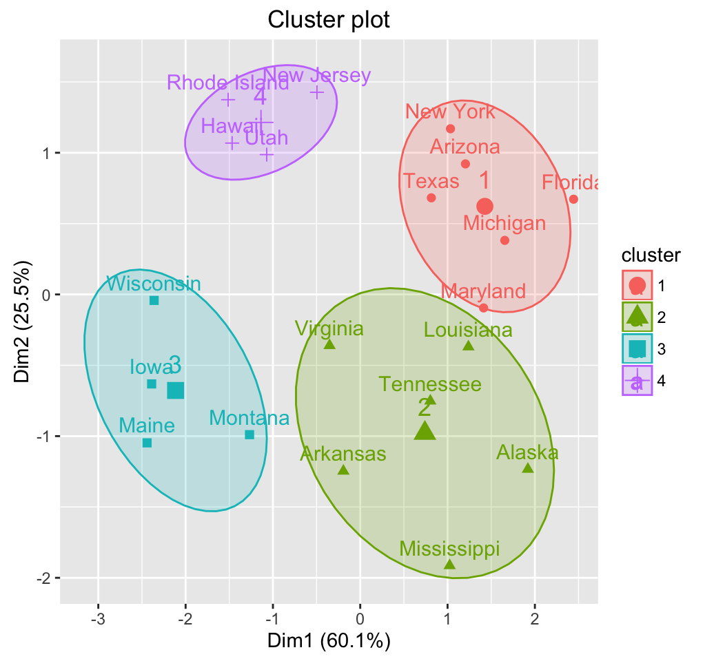
## [6] "withinerror" "call"fviz_cluster(list(data = df, cluster=cm$cluster), frame.type = "norm",
frame.level = 0.68)
4 Infos
This analysis has been performed using R software (ver. 3.2.4)
- J. C. Dunn (1973): A Fuzzy Relative of the ISODATA Process and Its Use in Detecting Compact Well-Separated Clusters. Journal of Cybernetics 3: 32-57
- J. C. Bezdek (1981): Pattern Recognition with Fuzzy Objective Function Algorithms. Plenum Press, New York Tariq Rashid: Clustering