- 1 Introduction
- 2 How this document is organized?
- 3 Data preparation
- 4 Installing and loading required R packages
- 5 Clarifying distance measures
- 6 Basic clustering methods
- 7 Clustering validation
- 8 The guide for clustering analysis on a real data: 4 steps you should know
- 9 Visualization of clustering results
- 10 Advanced clustering methods
- 11 Infos
1 Introduction
1.1 Quick overview of machine learning
A huge amounts of multidimensional data have been collected in various fields such as marketing, bio-medical and geo-spatial fields. Mining knowledge from these big data becomes a highly demanding field. However, it far exceeded humans ability to analyze these huge data. Unsupervised Machine Learning or clustering is one of the important data mining methods for discovering knowledge in multidimensional data.
Machine learning (ML) is divided into two different fields:
- Supervised ML defined as a set of tools used for prediction (linear model, logistic regression, linear discriminant analysis, classification trees, support vector machines and more)
- Unsupervised ML, also known as clustering, is an exploratory data analysis technique used for identifying groups (i.e clusters) in the data set of interest. Each group contains observations with similar profile according to a specific criteria. Similarity between observations is defined using some inter-observation distance measures including Euclidean and correlation-based distance measures.
This document describes the use of unsupervised machine learning approaches, including Principal Component Analysis (PCA) and clustering methods.
- Principal Component Analysis (PCA) is a dimension reduction techniques applied for simplifying the data and for visualizing the most important information in the data set
- Clustering is applied for identifying groups (i.e clusters) among the observations. Clustering can be subdivided into five general strategies:
- Partitioning methods
- Hierarchical clustering
- Fuzzy clustering
- Density-based clustering
- Model-based clustering
Note that, it possible to cluster both observations (i.e, samples or individuals) and features (i.e, variables). Observations can be clustered on the basis of variables and variables can be clustered on the basis of observations.
1.2 Applications of unsupervised machine learning
Unsupervised ML is popular in many fields, including:
- In cancer research field in order to classify patients in subgroups according their gene expression profile. This can be useful for identifying the molecular profile of patients with good or bad prognostic, as well as for understanding the disease.
- In marketing for market segmentation by identifying subgroups of customers with similar profiles and who might be receptive to a particular form of advertising.
- City-planning: for identifying groups of houses according to their type, value and location.
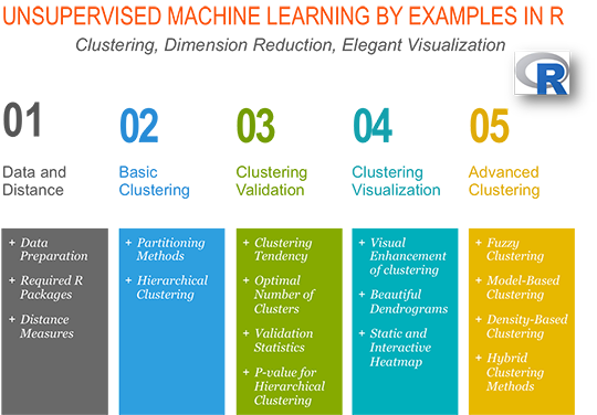
2 How this document is organized?
Here,
- we start by describing the two standard clustering strategies [partitioning methods (k-MEANS, PAM, CLARA) and hierarchical clustering] as well as how to assess the quality of clustering analysis.
- next, we provide a step-by-step guide for clustering analysis and an R package, named factoextra, for ggplot2-based elegant clustering visualization.
- finally, we describe advanced clustering approaches to find pattern of any shape in large data sets with noise and outliers.
Data preparation
Installing and loading required R packages
- Basic clustering methods
- Partitioning Cluster Analysis
- Hierarchical Clustering Essentials
- Evaluation of clustering
The guide for clustering analysis on a real data: 4 steps you should know?
- Elegant Clustering Visualization
- Visual enhancement of clustering analysis
- Beautiful dendrogram visualizations in R: 5+ must known methods
- Static and Interactive Heatmap in R
- Advanced Clustering Methods
- Fuzzy clustering analysis
- Model-Based Clustering
- DBSCAN: density-based clustering for discovering clusters in large datasets with noise
- Hybrid hierarchical k-means clustering for optimizing clustering outputs - Hybrid approach (1/1)
- HCPC: Hierarchical clustering on principal components - Hybrid approach (2/2)
- Clustering on categorical variables: CA, MCA > HCPC (coming soon)
To be published late in 2016. Subscribe to our mailing list at: STHDA mailing list. You will be notified about this book.
This work is licensed under the Creative Commons Attribution-NonCommercial-NoDerivs 3.0 United States License.
3 Data preparation
The built-in R dataset USArrest is used as demo data.
- Remove missing data
- Scale variables to make them comparable
# Load data
data("USArrests")
my_data <- USArrests

# Remove any missing value (i.e, NA values for not available)
my_data <- na.omit(my_data)

# Scale variables
my_data <- scale(my_data)

# View the firt 3 rows
head(my_data, n = 3)
## Murder Assault UrbanPop Rape
## Alabama 1.24256408 0.7828393 -0.5209066 -0.003416473
## Alaska 0.50786248 1.1068225 -1.2117642 2.484202941
## Arizona 0.07163341 1.4788032 0.9989801 1.0428783884 Installing and loading required R packages
- Install required packages
- cluster: for computing clustering
- factoextra: for elegant ggplot2-based data visualization. See the online documentation at: http://www.sthda.com/english/rpkgs/factoextra/
# Install factoextra
install.packages("factoextra")

# Install cluster package
install.packages("cluster")- Loading required packages
library("cluster")
library("factoextra")
5 Clarifying distance measures
In this chapter, we covered the common distance measures used for assessing similarity between observations. Some R codes, for computing and visualizing pairwise-distances between observations, are also provided.
How this chapter is organized?
- Methods for measuring distances
- Distances and scaling
- Data preparation
- R functions for computing distances
- The standard dist() function
- Correlation based distance measures
- The function daisy() in cluster package
- Visualizing distance matrices
Read more: Clarifying distance measures.
Its simple to compute and visualize distance matrix using the functions get_dist() and fviz_dist() in factoextra R package:
get_dist(): for computing a distance matrix between the rows of a data matrix. Compared to the standard dist() function, it supports correlation-based distance measures including pearson, kendall and spearman methods.
fviz_dist(): for visualizing a distance matrix
res.dist <- get_dist(USArrests, stand = TRUE, method = "pearson")

fviz_dist(res.dist,
   gradient = list(low = "#00AFBB", mid = "white", high = "#FC4E07"))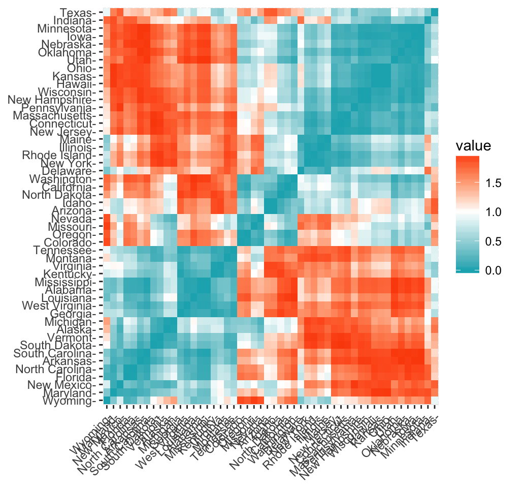
Clustering - Unsupervised Machine Learning
Read more: Clarifying distance measures.
6 Basic clustering methods
6.1 Partitioning clustering
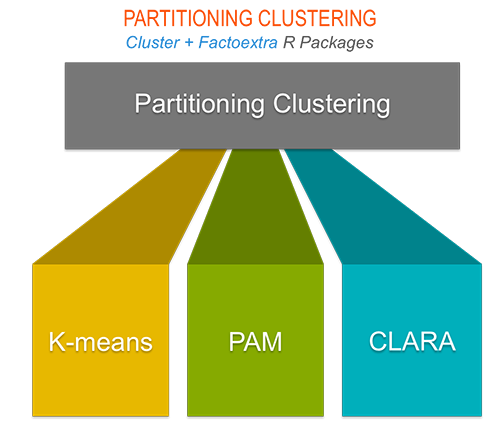
This chapter describes the most commonly used partitioning algorithms including:
- K-means clustering (MacQueen, 1967), in which, each cluster is represented by the center or means of the data points belonging to the cluster.
- K-medoids clustering or PAM (Partitioning Around Medoids, Kaufman & Rousseeuw, 1990), in which, each cluster is represented by one of the objects in the cluster. Its a non-parametric alternative of k-means clustering. Well describe also a variant of PAM named CLARA (Clustering Large Applications) which is used for analyzing large data sets.
For each of these methods, we provide:
- the basic idea and the key mathematical concepts
- the clustering algorithm and implementation in R software
- R lab sections with many examples for computing clustering methods and visualizing the outputs
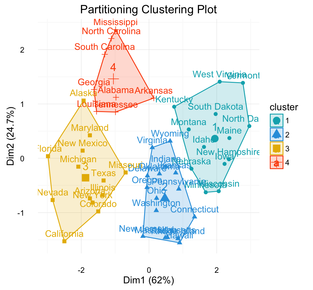
Clustering - Unsupervised Machine Learning
How this chapter is organized?
- Required packages: cluster (for computing clustering algorithm) and factoextra (for elegant visualization)
- K-means clustering
- Concept
- Algorithm
- R function for k-means clustering: stats::kmeans()
- Data format
- Compute k-means clustering
- Application of K-means clustering on real data
- Data preparation and descriptive statistics
- Determine the number of optimal clusters in the data: factoextra::fviz_nbclust()
- Compute k-means clustering
- Plot the result: factoextra::fviz_cluster()
- PAM: Partitioning Around Medoids
- Concept
- Algorithm
- R function for computing PAM: cluster::pam() or fpc::pamk()
- Compute PAM
- CLARA: Clustering Large Applications
- Concept
- Algorithm
- R function for computing CLARA: cluster::clara()
- R packages and functions for visualizing partitioning clusters
- cluster::clusplot() function
- factoextra::fviz_cluster() function
Read more: Partitioning cluster analysis. If you are in hurry, read the following quick-start guide.
- K-means clustering: split the data into a set of k groups (i.e., cluster), where k must be specified by the analyst. Each cluster is represented by means of points belonging to the cluster.
Determine the optimal number of clusters: use factoextra::fviz_nbclust()
library("factoextra")
fviz_nbclust(my_data, kmeans, method = "gap_stat")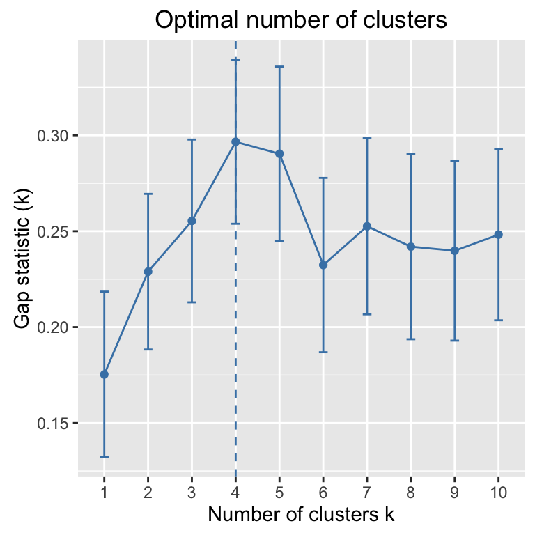
Clustering - Unsupervised Machine Learning
Compute and visualize k-means clustering
km.res <- kmeans(my_data, 4, nstart = 25)

# Visualize
library("factoextra")
fviz_cluster(km.res, data = my_data, frame.type = "convex")+
  theme_minimal()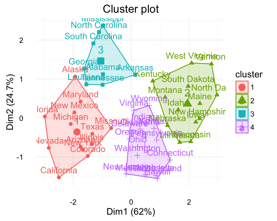
Clustering - Unsupervised Machine Learning
- PAM clustering: Partitioning Around Medoids. Robust alternative to k-means clustering, less sensitive to outliers.
# Compute PAM
library("cluster")
pam.res <- pam(my_data, 4)

# Visualize
fviz_cluster(pam.res)
Read more: Partitioning cluster analysis.
6.2 Hierarchical clustering
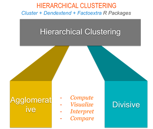
Hierarchical clustering can be subdivided into two types:
- Agglomerative hierarchical clustering (AHC) in which, each observation is initially considered as a cluster of its own (leaf. Then, the most similar clusters are iteratively merged until there is just one single big cluster (root).
- Divise hierarchical clustering which is an inverse of AHC. It begins with the root, in witch all objects are included in one cluster. Then the most heterogeneous clusters are iteratively divided until all observation are in their own cluster.
The result of hierarchical clustering is a tree-based representation of the observations which is called a dendrogram. Observations can be subdivided into groups by cutting the dendogram at a desired similarity level.
This chapter provides:
- The description of the different types of hierarchical clustering algorithms
- R lab sections with many examples for computing hierarchical clustering, visualizing and comparing dendrogram
- The interpretation of dendrogram
- R codes for cutting the dendrograms into groups
How this chapter is organized?
- Required R packages
- Algorithm
- Data preparation and descriptive statistics
- R functions for hierarchical clustering
- hclust() function
- agnes() and diana() functions
- Interpretation of the dendrogram
- Cut the dendrogram into different groups
- Hierarchical clustering and correlation based distance
- What type of distance measures should we choose?
- Comparing two dendrograms
- Tanglegram
- Correlation matrix between a list of dendrogram
Read more: Hierarchical clustering essentials. If you are in hurry, read the following quick-start guide.
Install and load required packages (cluster, factoextra) as previously described
Compute and visualize hierarchical clustering using R base functions
# 1. Loading and preparing data
data("USArrests")
my_data <- scale(USArrests)

# 2. Compute dissimilarity matrix
d <- dist(my_data, method = "euclidean")

# Hierarchical clustering using Ward's method
res.hc <- hclust(d, method = "ward.D2" )

# Cut tree into 4 groups
grp <- cutree(res.hc, k = 4)

# Visualize
plot(res.hc, cex = 0.6) # plot tree
rect.hclust(res.hc, k = 4, border = 2:5) # add rectangle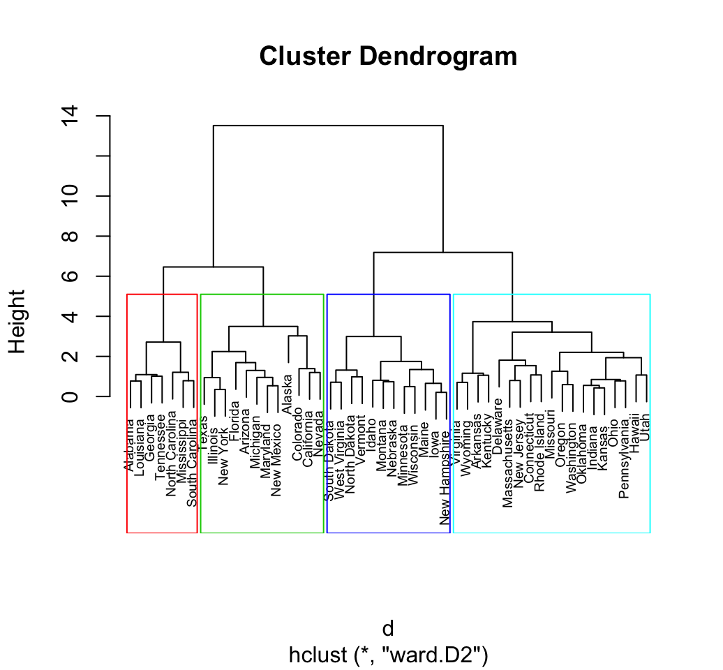
Clustering - Unsupervised Machine Learning
- Elegant visualization using factoextra functions: factoextra::hcut(), factoextra::fviz_dend()
library("factoextra")
# Compute hierarchical clustering and cut into 4 clusters
res <- hcut(USArrests, k = 4, stand = TRUE)

# Visualize
fviz_dend(res, rect = TRUE, cex = 0.5,
          k_colors = c("#00AFBB","#2E9FDF", "#E7B800", "#FC4E07"))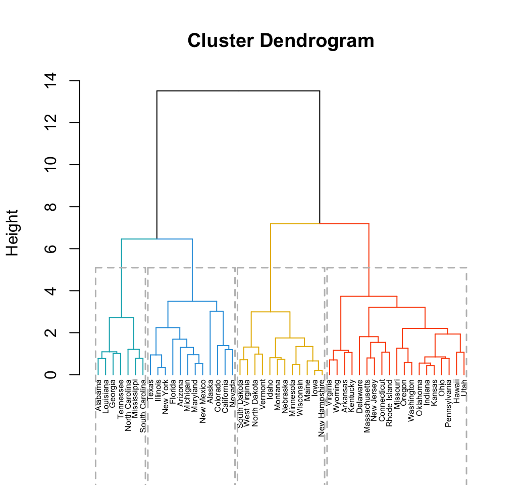
Clustering - Unsupervised Machine Learning
Well see also, how to customize the dendrogram:
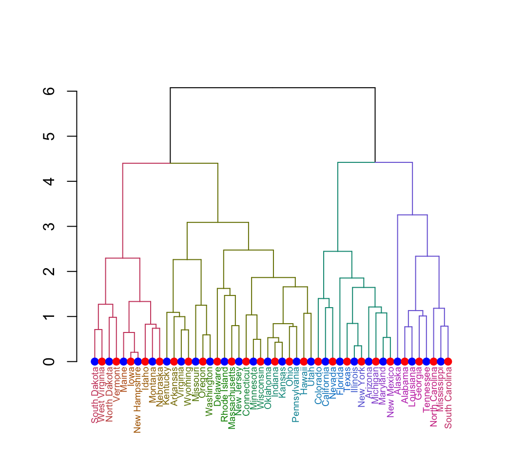
Clustering - Unsupervised Machine Learning
Read more: Hierarchical clustering essentials.
7 Clustering validation
Clustering validation includes three main tasks:
- clustering tendency assesses whether applying clustering is suitable to your data.
- clustering evaluation assesses the goodness or quality of the clustering.
- clustering stability seeks to understand the sensitivity of the clustering result to various algorithmic parameters, for example, the number of clusters.
The aim of this part is to:
- describe the different methods for clustering validation
- compare the quality of clustering results obtained with different clustering algorithms
- provide R lab section for validating clustering results
7.1 Assessing clustering tendency
In this chapter:
- We describe why we should evaluate the clustering tendency before applying any cluster analysis on a dataset.
- We describe statistical and visual methods for assessing the clustering tendency
- R lab sections containing many examples are also provided for computing clustering tendency and visualizing clusters
How this chapter is organized?
- Required packages
- Data preparation
- Why assessing clustering tendency?
- Methods for assessing clustering tendency
- Hopkins statistic
- Algorithm
- R function for computing Hopkins statistic: clustertend::hopkins()
- VAT: Visual Assessment of cluster Tendency: seriation::dissplot()
- VAT Algorithm
- R functions for VAT
- Hopkins statistic
- A single function for Hopkins statistic and VAT: factoextra::get_clust_tendency()
Read more: Assessing clustering tendency. If you are in hurry, read the following quick-start guide.
Install and load factoextra as previously described
Assessing clustering tendency: use factoextra::get_clust_tendency(). Assess clustering tendency using Hopkins statistic and a visual approach. An ordered dissimilarity image (ODI) is shown.
Hopkins statistic: If the value of Hopkins statistic is close to zero (far below 0.5), then we can conclude that the dataset is significantly clusterable.
- VAT (Visual Assessment of cluster Tendency): The VAT detects the clustering tendency in a visual form by counting the number of square shaped dark (or colored) blocks along the diagonal in a VAT image.
library("factoextra")
my_data <- scale(iris[, -5])
get_clust_tendency(my_data, n = 50,
                   gradient = list(low = "steelblue",  high = "white"))
## $hopkins_stat
## [1] 0.2002686
##
## $plot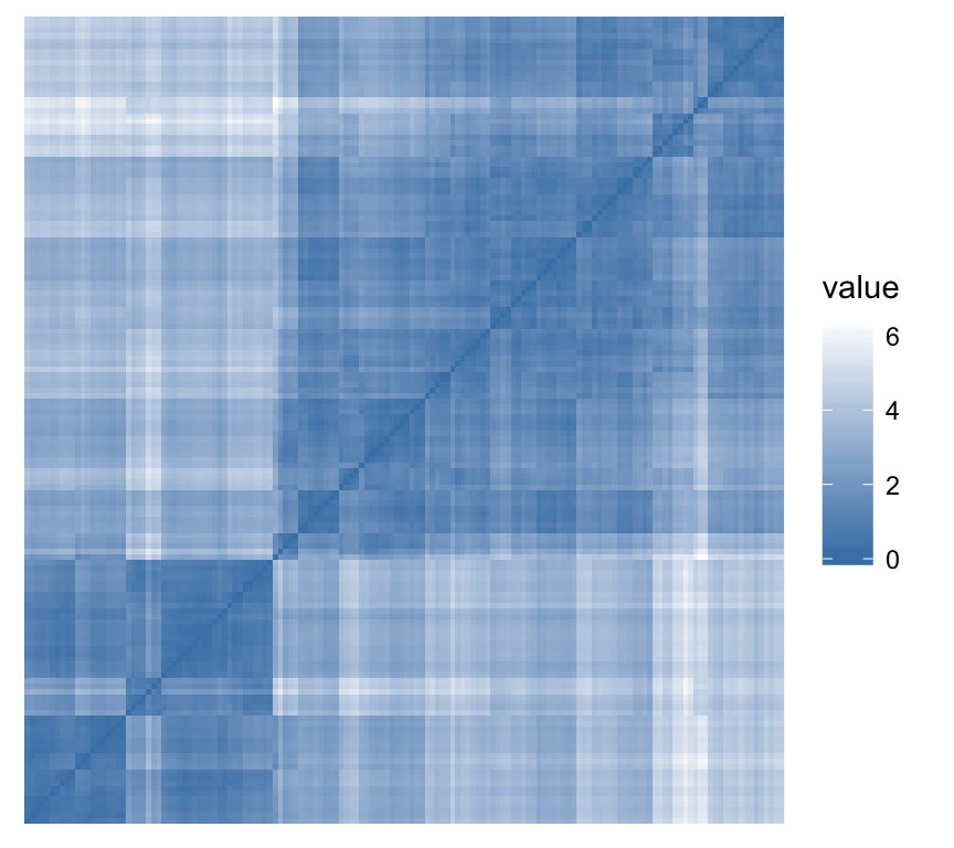
Clustering - Unsupervised Machine Learning
Read more: Assessing clustering tendency.
7.2 Determining the optimal number of clusters
In this chapter, well describe different methods to determine the optimal number of clusters for k-means, PAM and hierarchical clustering.
How this chapter is organized?
- Required packages
- Data preparation
- Example of partitioning method results
- Example of hierarchical clustering results
- Three popular methods for determining the optimal number of clusters
- Elbow method
- Concept
- Algorithm
- R codes
- Average silhouette method
- Concept
- Algorithm
- R codes
- Conclusions about elbow and silhouette methods
- Gap statistic method
- Concept
- Algorithm
- R codes
- Elbow method
- NbClust: A Package providing 30 indices for determining the best number of clusters
- Overview of NbClust package
- NbClust R function
- Examples of usage
- Compute only an index of interest
- Compute all the 30 indices
Read more: Determining the optimal number of clusters. If you are in hurry, read the following quick-start guide.
- Estimate the number of clusters in the data using gap statistics : factoextra::fviz_nbclust()
my_data <- scale(USArrests)
library("factoextra")
fviz_nbclust(my_data, kmeans, method = "gap_stat")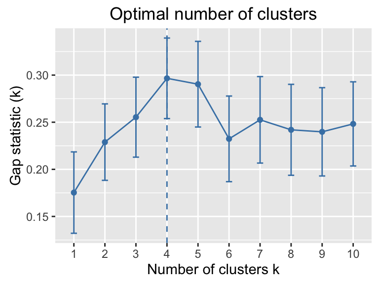
Clustering - Unsupervised Machine Learning
- NbClust: A Package providing 30 indices for determining the best number of clusters
library("NbClust")
set.seed(123)
res.nbclust <- NbClust(my_data, distance = "euclidean",
                  min.nc = 2, max.nc = 10,
                  method = "complete", index ="all")
Visualize using factoextra:
factoextra::fviz_nbclust(res.nbclust) + theme_minimal()## Among all indices:
## ===================
## * 2 proposed 0 as the best number of clusters
## * 1 proposed 1 as the best number of clusters
## * 9 proposed 2 as the best number of clusters
## * 4 proposed 3 as the best number of clusters
## * 6 proposed 4 as the best number of clusters
## * 2 proposed 5 as the best number of clusters
## * 1 proposed 8 as the best number of clusters
## * 1 proposed 10 as the best number of clusters
##
## Conclusion
## =========================
## * According to the majority rule, the best number of clusters is 2 .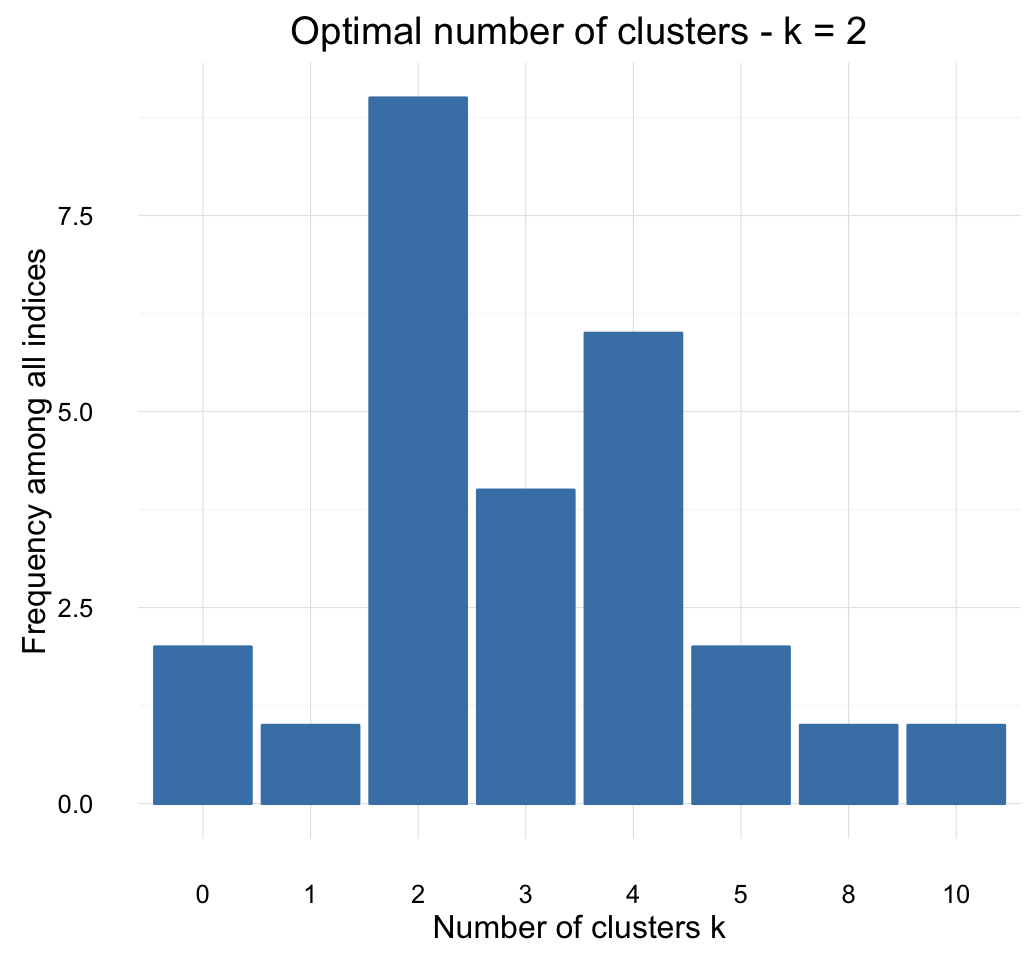
Clustering - Unsupervised Machine Learning
Read more: Determining the optimal number of clusters.
7.3 Clustering validation statistics
The aim of this chapter is to:
- describe the different methods for clustering validation
- compare the quality of clustering results obtained with different clustering algorithms
- provide R lab section for validating clustering results
How this chapter is organized?
- Required packages: cluster, factoextra, NbClust, fpc
- Data preparation
- Relative measures - Determine the optimal number of clusters: NbClust::NbClust()
- Clustering analysis
- Example of partitioning method results
- Example of hierarchical clustering results
- Internal clustering validation measures
- Silhouette analysis
- Concept and algorithm
- Interpretation of silhouette width
- R functions for silhouette analysis: cluster::silhouette(), factoextra::fviz_silhouette()
- Dunn index
- Concept and algorithm
- R function for computing Dunn index: fpc::cluster.stats(), NbClust::NbClust()
- Clustering validation statistics: fpc::cluster.stats()
- Silhouette analysis
- External clustering validation
Read more: Clustering Validation Statistics. If you are in hurry, read the following quick-start guide.
- Compute and visualize hierarchical clustering
- Compute: factoextra::eclust()
- Elegant visualization: factoextra::fviz_dend()
my_data <- scale(iris[, -5])

# Enhanced hierarchical clustering, cut in 3 groups
library("factoextra")
res.hc <- eclust(my_data, "hclust", k = 3, graph = FALSE)

# Visualize
fviz_dend(res.hc, rect = TRUE, show_labels = FALSE)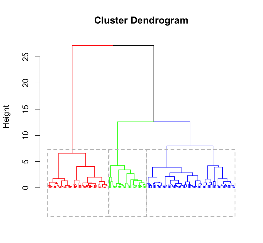
Clustering - Unsupervised Machine Learning
- Validate clustering results by inspection the cluster silhouette plot
Recall that the silhouette (\(S_i\)) measures how similar an object \(i\) is to the the other objects in its own cluster versus those in the neighbor cluster. \(S_i\) values range from 1 to - 1:
- A value of \(S_i\) close to 1 indicates that the object is well clustered. In the other words, the object \(i\) is similar to the other objects in its group.
- A value of \(S_i\) close to -1 indicates that the object is poorly clustered, and that assignment to some other cluster would probably improve the overall results.
# Visualize the silhouette plot
fviz_silhouette(res.hc)
## cluster size ave.sil.width
## 1 1 49 0.63
## 2 2 30 0.44
## 3 3 71 0.32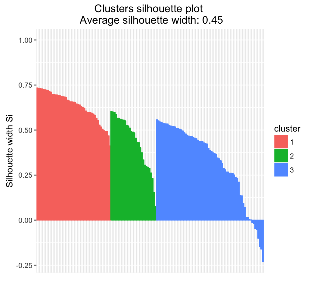
Clustering - Unsupervised Machine Learning
Which samples have negative silhouette? To what cluster are they closer?
# Silhouette width of observations
sil <- res.hc$silinfo$widths[, 1:3]

# Objects with negative silhouette
neg_sil_index <- which(sil[, 'sil_width'] < 0)
sil[neg_sil_index, , drop = FALSE]
## cluster neighbor sil_width
## 84 3 2 -0.01269799
## 122 3 2 -0.01789603
## 62 3 2 -0.04756835
## 135 3 2 -0.05302402
## 73 3 2 -0.10091884
## 74 3 2 -0.14761137
## 114 3 2 -0.16107155
## 72 3 2 -0.23036371
Read more: Clustering Validation Statistics.
7.4 How to choose the appropriate clustering algorithms for your data?
Well start by describing the different clustering validation measures in the package. Next, well present the function clValid() and finally well provide an R lab section for validating clustering results and comparing clustering algorithms.
How this chapter is organized?
- Clustering validation measures in clValid package
- Internal validation measures
- Stability validation measures
- Biological validation measures
- R function clValid()
- Format
- Examples of usage
- Data
- Compute clValid()
Read more: How to choose the appropriate clustering algorithms for your data?. If you are in hurry, read the following quick-start guide.
my_data <- scale(USArrests)

# Compute clValid
library("clValid")
intern <- clValid(my_data, nClust = 2:6,
              clMethods = c("hierarchical","kmeans","pam"),
              validation = "internal")
# Summary
summary(intern)
##
## Clustering Methods:
## hierarchical kmeans pam
##
## Cluster sizes:
## 2 3 4 5 6
##
## Validation Measures:
## 2 3 4 5 6
##
## hierarchical Connectivity 6.6437 9.5615 13.9563 22.5782 31.2873
## Dunn 0.2214 0.2214 0.2224 0.2046 0.2126
## Silhouette 0.4085 0.3486 0.3637 0.3213 0.2720
## kmeans Connectivity 6.6437 13.6484 16.2413 24.6639 33.7194
## Dunn 0.2214 0.2224 0.2224 0.1983 0.2231
## Silhouette 0.4085 0.3668 0.3573 0.3377 0.3079
## pam Connectivity 6.6437 13.8302 20.4421 29.5726 38.2643
## Dunn 0.2214 0.1376 0.1849 0.1849 0.2019
## Silhouette 0.4085 0.3144 0.3390 0.3105 0.2630
##
## Optimal Scores:
##
## Score Method Clusters
## Connectivity 6.6437 hierarchical 2
## Dunn 0.2231 kmeans 6
## Silhouette 0.4085 hierarchical 2It can be seen that hierarchical clustering with two clusters performs the best in each case (i.e., for connectivity, Dunn and Silhouette measures).
Read more: How to choose the appropriate clustering algorithms for your data?.
7.5 How to compute p-value for hierarchical clustering in R?
How this chapter is organized?
- Concept
- Algorithm
- Required R packages
- Data preparation
- Compute p-value for hierarchical clustering
- Description of pvclust() function
- Usage of pvclust() function
Read more: How to compute p-value for hierarchical clustering in R?. If you are in hurry, read the following quick-start guide.
Note that, pvclust() performs clustering on the columns of the dataset, which correspond to samples in our case.
library(pvclust)
# Data preparation
set.seed(123)
data("lung")
ss <- sample(1:73, 30) # extract 20 samples out of
my_data <- lung[, ss]
# Compute pvclust
res.pv <- pvclust(my_data, method.dist="cor",
method.hclust="average", nboot = 10)## Bootstrap (r = 0.5)... Done.
## Bootstrap (r = 0.6)... Done.
## Bootstrap (r = 0.7)... Done.
## Bootstrap (r = 0.8)... Done.
## Bootstrap (r = 0.9)... Done.
## Bootstrap (r = 1.0)... Done.
## Bootstrap (r = 1.1)... Done.
## Bootstrap (r = 1.2)... Done.
## Bootstrap (r = 1.3)... Done.
## Bootstrap (r = 1.4)... Done.# Default plot
plot(res.pv, hang = -1, cex = 0.5)
pvrect(res.pv)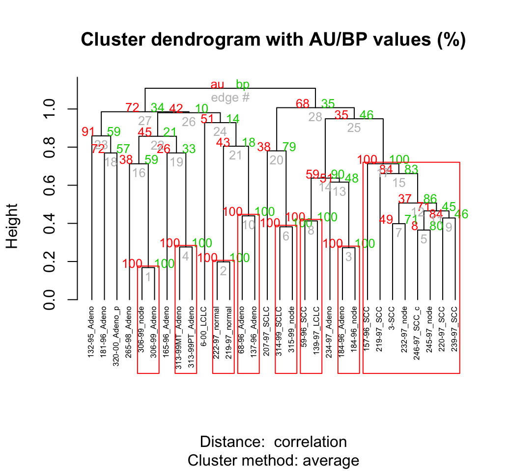
Clustering - Unsupervised Machine Learning
Clusters with AU > = 95% are indicated by the rectangles and are considered to be strongly supported by data.
Read more: How to compute p-value for hierarchical clustering in R?.
8 The guide for clustering analysis on a real data: 4 steps you should know
In this chapter well describe the different steps to follow for computing clustering on a real data using k-means clustering:
Read more: The guide for clustering analysis on a real data: 4 steps you should know.
9 Visualization of clustering results
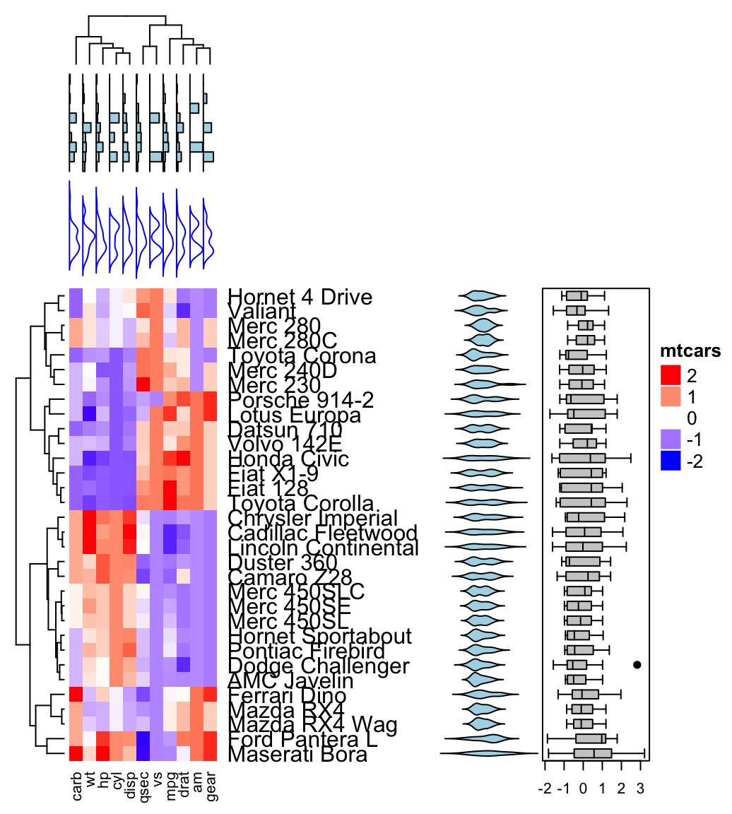
In this chapter, well describe how to visualize the result of clustering using dendrograms as well as static and interactiveheatmap.
Heat map is a false color image with a dendrogram added to the left side and to the top. Its used to visualize a hidden pattern in a data matrix in order to reveal some associations between rows or columns.
9.1 Visual enhancement of clustering analysis
Read more: Visual enhancement of clustering analysis.
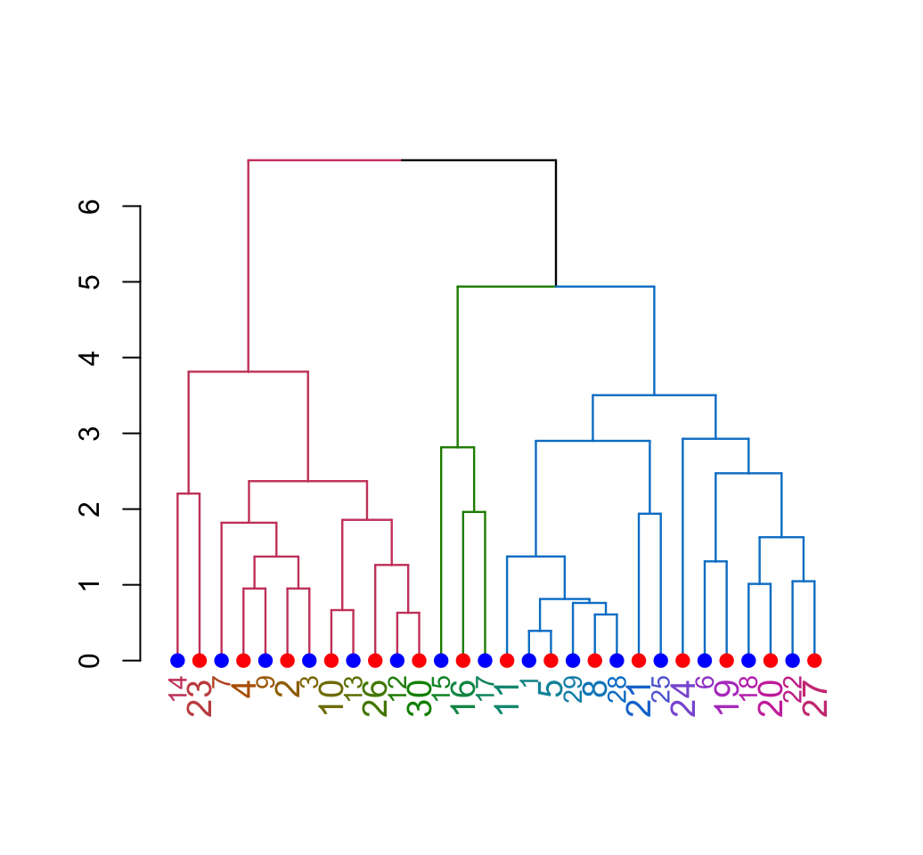
9.2 Beautiful dendrogram visualizations
Read more: Beautiful dendrogram visualizations in R: 5+ must known methods
Clustering - Unsupervised Machine Learning
9.3 Static and Interactive Heatmap
Read more: Static and Interactive Heatmap in R
Clustering - Unsupervised Machine Learning
10 Advanced clustering methods
10.1 Fuzzy clustering analysis
Fuzzy clustering is also known as soft method. Standard clustering approaches produce partitions (K-means, PAM), in which each observation belongs to only one cluster. This is known as hard clustering.
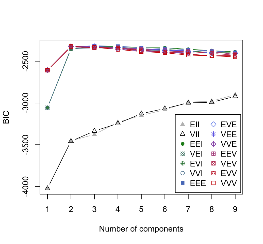
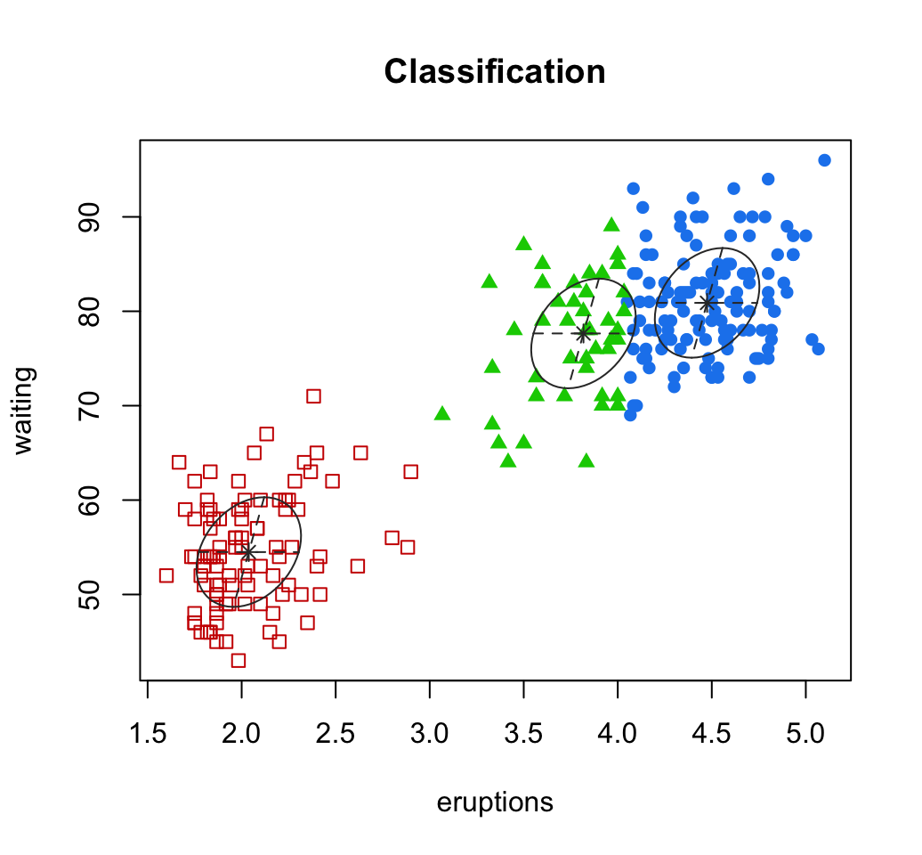
10.2 Model-based clustering
Clustering - Unsupervised Machine Learning
10.3 DBSCAN: Density-based clustering
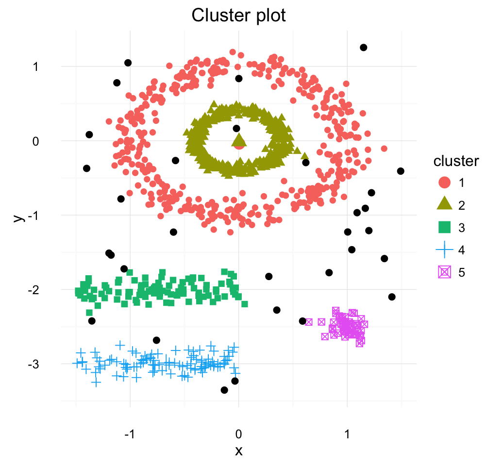
DBSCAN is a partitioning method that has been introduced in Ester et al. (1996). It can find out clusters of different shapes and sizes from data containing noise and outliers.The basic idea behind density-based clustering approach is derived from a human intuitive clustering method.
The description and implementation of DBSCAN in R are provided in this chapter : DBSCAN.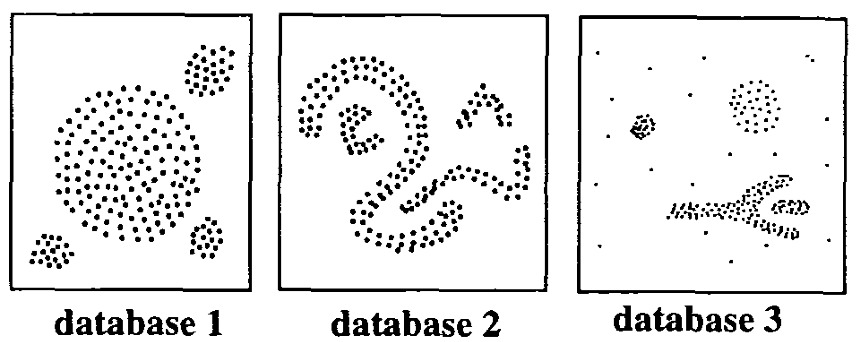
Clustering - Unsupervised Machine Learning
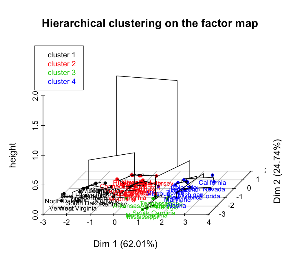
10.4 Hybrid clustering methods
- Hybrid hierarchical k-means clustering for optimizing clustering outputs - Hybrid approach (1/1)
- HCPC: Hierarchical clustering on principal components - Hybrid approach (2/2)
Clustering - Unsupervised Machine Learning
11 Infos
This analysis has been performed using R software (ver. 3.2.4)
- Martin Ester, Hans-Peter Kriegel, Joerg Sander, Xiaowei Xu (1996). A Density-Based Algorithm for Discovering Clusters in Large Spatial Databases with Noise. Institute for Computer Science, University of Munich. Proceedings of 2nd International Conference on Knowledge Discovery and Data Mining (KDD-96). pdf
