Previously, we described the essentials of R programming and provided quick start guides for importing data into R.
Here, well describe how to create histogram and density plots in R.
Pleleminary tasks
Launch RStudio as described here: Running RStudio and setting up your working directory
Prepare your data as described here: Best practices for preparing your data and save it in an external .txt tab or .csv files
Import your data into R as described here: Fast reading of data from txt|csv files into R: readr package.
Create some data
The data set contains the value of weight by sex for 200 individuals.
set.seed(1234)
x <- c(rnorm(200, mean=55, sd=5),
     rnorm(200, mean=65, sd=5))
head(x)
## [1] 48.96467 56.38715 60.42221 43.27151 57.14562 57.53028Create histogram plots: hist()
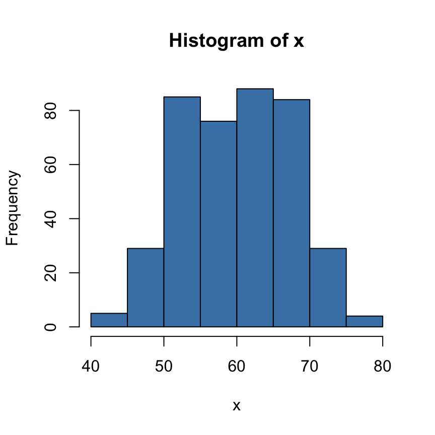
- A histogram can be created using the function hist(), which simplified format is as follow:
hist(x, breaks = "Sturges")- x: a numeric vector
- breaks: breakpoints between histogram cells.
- Create histograms
hist(x, col = "steelblue", frame = FALSE)
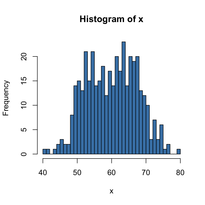
# Change the number of breaks
hist(x, col = "steelblue", frame = FALSE,
     breaks = 30)
Create density plots: density()
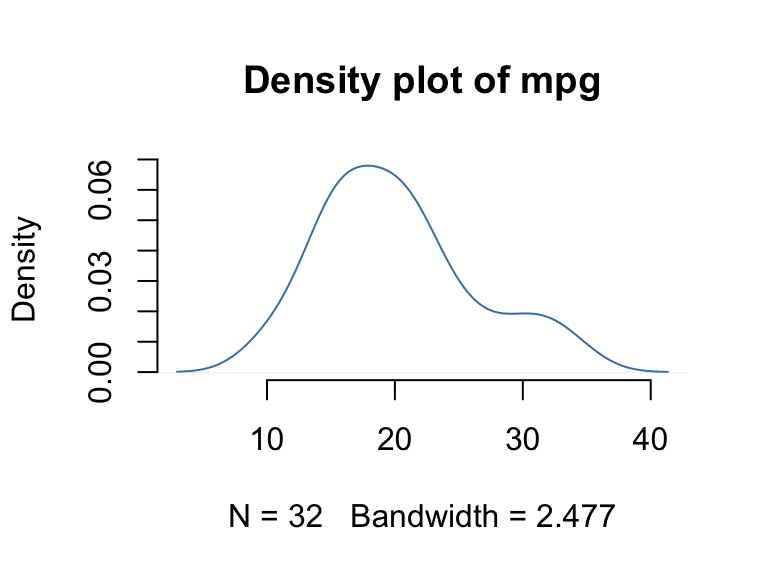
The function density() is used to estimate kernel density.
# Compute the density data
dens <- density(mtcars$mpg)
# plot density
plot(dens, frame = FALSE, col = "steelblue",
main = "Density plot of mpg") 
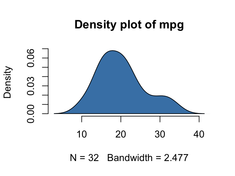
# Fill the density plot using polygon()
plot(dens, frame = FALSE, col = "steelblue",
     main = "Density plot of mpg")
polygon(dens, col = "steelblue")
See also
Infos
This analysis has been performed using R statistical software (ver. 3.2.4).